Working with Betweenness Centrality

The betweenness centrality of a graph is a measure of centrality based on shortest paths. For every pair of nodes in a connected graph, there is at least a single shortest path between the nodes such that the number of edges the path passes through is minimized. The betweenness centrality for a given graph node is the number of these shortest paths that pass through the node.

This is defined as:

\[c_B(v) =\sum_{s,t \in V} \frac{\sigma(s, t|v)}{\sigma(s, t)}\]

where \(V\) is the set of nodes, \(\sigma(s, t)\) is the number of shortest \((s, t)\) paths, and \(\sigma(s, t|v)\) is the number of those paths passing through some node \(v\) other than \(s, t\). If \(s = t\), \(\sigma(s, t) = 1\), and if \(v \in {s, t}\), \(\sigma(s, t|v) = 0\)

This tutorial will take you through the process of calculating the betweenness centrality of a graph and visualizing it.

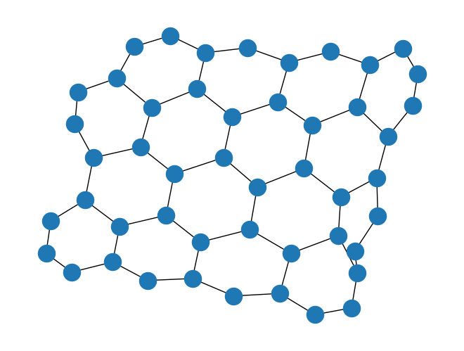
Generate a Graph

To start we need to generate a graph:

import rustworkx as rx
from rustworkx.visualization import mpl_draw

graph = rx.generators.hexagonal_lattice_graph(4, 4)
mpl_draw(graph)

Calculate the Betweeness Centrality

The betweenness_centrality() function can be used to calculate the betweenness centrality for each node in the graph.

import pprint

centrality = rx.betweenness_centrality(graph)
# Print the centrality value for the first 5 nodes in the graph
pprint.pprint({x: centrality[x] for x in range(5)})

{0: 0.007277212457600987,
 1: 0.02047046385621779,
 2: 0.07491079688119466,
 3: 0.04242324126690451,
 4: 0.09205321351482312}

The output of betweenness_centrality() is a CentralityMapping which is a custom mapping type that maps the node index to the centrality value as a float. This is a mapping and not a sequence because node indices (and edge indices too, which is not relevant here) are not guaranteed to be a contiguous sequence if there are removals.

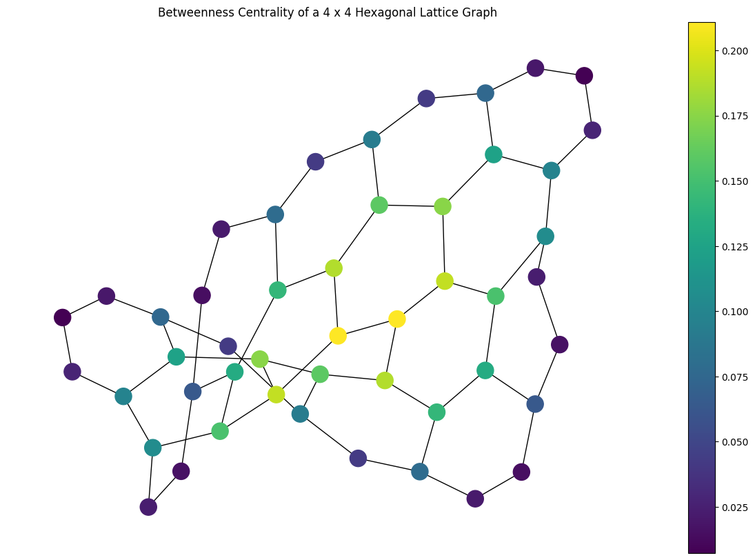
Visualize the Betweenness Centrality

Now that we’ve found the betweenness centrality for graph lets visualize it. We’ll color each node in the output visualization using its calculated centrality:

import matplotlib.pyplot as plt

# Generate a color list
colors = []
for node in graph.node_indices():
    colors.append(centrality[node])
# Generate a visualization with a colorbar
plt.rcParams['figure.figsize'] = [15, 10]
ax = plt.gca()
sm = plt.cm.ScalarMappable(norm=plt.Normalize(
    vmin=min(centrality.values()),
    vmax=max(centrality.values())
))
plt.colorbar(sm, ax=ax)
plt.title("Betweenness Centrality of a 4 x 4 Hexagonal Lattice Graph")
mpl_draw(graph, node_color=colors, ax=ax)

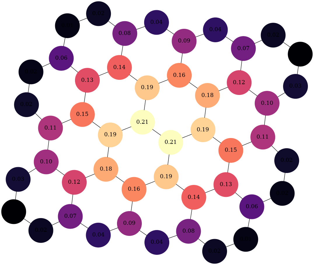
Alternatively, you can use graphviz_draw():

from rustworkx.visualization import graphviz_draw
import matplotlib

# For graphviz visualization we need to assign the data payload for each
# node to its centrality value so that we can color based on this
for node, btw in centrality.items():
    graph[node] = btw

# Leverage matplotlib for color map
colormap = matplotlib.colormaps["magma"]
norm = matplotlib.colors.Normalize(
    vmin=min(centrality.values()),
    vmax=max(centrality.values())
)

def color_node(node):
    rgba = matplotlib.colors.to_hex(colormap(norm(node)), keep_alpha=True)
    return {
        "color": f"\"{rgba}\"",
        "fillcolor": f"\"{rgba}\"",
        "style": "filled",
        "shape": "circle",
        "label": "%.2f" % node,
    }

graphviz_draw(graph, node_attr_fn=color_node, method="neato")