নোট
এই পৃষ্ঠাটি docs/tutorials/03_ground_state_solvers.ipynb থেকে বানানো হয়েছে।
গ্রাউন্ড স্টেট সমাধানকারী#
ভূমিকা#
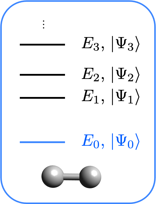
In this tutorial we are going to discuss the ground state calculation interface of Qiskit Nature. The goal is to compute the ground state of a molecular Hamiltonian. This Hamiltonian can for example be electronic or vibrational. To know more about the preparation of the Hamiltonian, check out the Electronic structure and Vibrational structure tutorials.
It should be said, that in the electronic case, we are actually computing purely the electronic part. When using the Qiskit Nature stack as presented in this tutorial, the nuclear repulsion energy will be added automatically, to obtain the total ground state energy.
প্রথম ধাপ হল আণবিক সিস্টেমকে সংজ্ঞায়িত করা। নিচে আমরা হাইড্রোজেন অণুর বৈদ্যুতিক অংশটি পেতে চাই।
[1]:
from qiskit_nature.units import DistanceUnit
from qiskit_nature.second_q.drivers import PySCFDriver

driver = PySCFDriver(
    atom="H 0 0 0; H 0 0 0.735",
    basis="sto3g",
    charge=0,
    spin=0,
    unit=DistanceUnit.ANGSTROM,
)

es_problem = driver.run()
We will also be sticking to the Jordan-Wigner mapping. To learn more about the various mappers available in Qiskit Nature, check out the Qubit Mappers tutorial.
[2]:
from qiskit_nature.second_q.mappers import JordanWignerMapper

mapper = JordanWignerMapper()
সমাধানকারী (The Solver)#
After these steps, we need to define a solver. The solver is the algorithm through which the ground state is computed.
Let’s first start with a purely classical example: the NumPyMinimumEigensolver. This algorithm exactly diagonalizes the Hamiltonian. Although it scales badly, it can be used on small systems to check the results of the quantum algorithms.
[3]:
from qiskit_algorithms import NumPyMinimumEigensolver

numpy_solver = NumPyMinimumEigensolver()
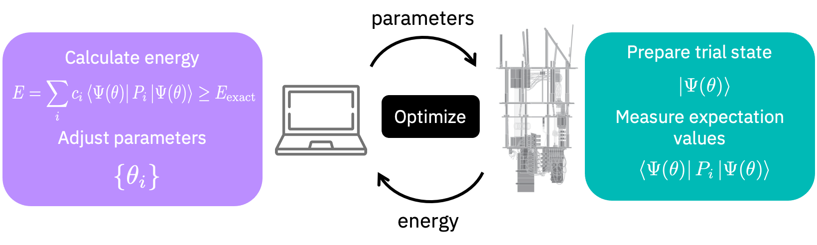
To find the ground state we could also use the Variational Quantum Eigensolver (VQE) algorithm. The VQE algorithm works by exchanging information between a classical and a quantum computer as depicted in the following figure.
Let’s initialize a VQE solver.
[4]:
from qiskit_algorithms import VQE
from qiskit_algorithms.optimizers import SLSQP
from qiskit.primitives import Estimator
from qiskit_nature.second_q.circuit.library import HartreeFock, UCCSD

ansatz = UCCSD(
    es_problem.num_spatial_orbitals,
    es_problem.num_particles,
    mapper,
    initial_state=HartreeFock(
        es_problem.num_spatial_orbitals,
        es_problem.num_particles,
        mapper,
    ),
)

vqe_solver = VQE(Estimator(), ansatz, SLSQP())
vqe_solver.initial_point = [0.0] * ansatz.num_parameters
To define the VQE solver one needs three essential elements:
An Estimator primitive: these were released as part of Qiskit Terra 0.22. To learn more about primitives, check out this resource.
A variational form: here we use the Unitary Coupled Cluster (UCC) ansatz (see for instance [Physical Review A 98.2 (2018): 022322]). Since it is a chemistry standard, a factory is already available allowing a fast initialization of a VQE with UCC. The default is to use all single and double excitations. However, the excitation type (S, D, SD) as well as other parameters can be selected. We also prepend the
UCCSDvariational form with aHartreeFockinitial state, which initializes the occupation of our qubits according to the problem which we are trying solve.An optimizer: this is the classical piece of code in charge of optimizing the parameters in our variational form. See the corresponding documentation for more information.
One could also use any available ansatz / initial state or even define one’s own. For instance,
[5]:
from qiskit_algorithms import VQE
from qiskit.circuit.library import TwoLocal

tl_circuit = TwoLocal(
    rotation_blocks=["h", "rx"],
    entanglement_blocks="cz",
    entanglement="full",
    reps=2,
    parameter_prefix="y",
)

another_solver = VQE(Estimator(), tl_circuit, SLSQP())
গননা এবং ফলাফল।#
We are now ready to put everything together to compute the ground-state of our problem. Doing so requires us to wrap our mapper and quantum algorithm into a single GroundStateEigensolver like so:
[6]:
from qiskit_nature.second_q.algorithms import GroundStateEigensolver

calc = GroundStateEigensolver(mapper, vqe_solver)
This will now take of the entire workflow: 1. generating the second-quantized operators stored in our problem (here referred to as es_problem) 2. mapping (and potentially reducing) the operators in the qubit space 3. running the quantum algorithm on the Hamiltonian qubit operator 4. once converged, evaluating the additional observables at the determined ground state
[7]:
res = calc.solve(es_problem)
print(res)
=== GROUND STATE ENERGY ===

* Electronic ground state energy (Hartree): -1.857275030145
  - computed part:      -1.857275030145
~ Nuclear repulsion energy (Hartree): 0.719968994449
> Total ground state energy (Hartree): -1.137306035696

=== MEASURED OBSERVABLES ===

  0:  # Particles: 2.000 S: 0.000 S^2: 0.000 M: 0.000

=== DIPOLE MOMENTS ===

~ Nuclear dipole moment (a.u.): [0.0  0.0  1.3889487]

  0:
  * Electronic dipole moment (a.u.): [0.0  0.0  1.38894893]
    - computed part:      [0.0  0.0  1.38894893]
  > Dipole moment (a.u.): [0.0  0.0  -0.00000023]  Total: 0.00000023
                 (debye): [0.0  0.0  -0.00000058]  Total: 0.00000058
আমরা ভি কিউ ই ফলাফল এর সাথে নামপাই এক্সাক্ট সমাধানকারীর (সলভার) তুলনা করতে পারি এবং দেখতে পারি তারা পরস্পর সমান কিনা।
[8]:
calc = GroundStateEigensolver(mapper, numpy_solver)
res = calc.solve(es_problem)
print(res)
=== GROUND STATE ENERGY ===

* Electronic ground state energy (Hartree): -1.857275030202
  - computed part:      -1.857275030202
~ Nuclear repulsion energy (Hartree): 0.719968994449
> Total ground state energy (Hartree): -1.137306035753

=== MEASURED OBSERVABLES ===

  0:  # Particles: 2.000 S: 0.000 S^2: 0.000 M: 0.000

=== DIPOLE MOMENTS ===

~ Nuclear dipole moment (a.u.): [0.0  0.0  1.3889487]

  0:
  * Electronic dipole moment (a.u.): [0.0  0.0  1.3889487]
    - computed part:      [0.0  0.0  1.3889487]
  > Dipole moment (a.u.): [0.0  0.0  0.0]  Total: 0.0
                 (debye): [0.0  0.0  0.0]  Total: 0.0
একটি ফিল্টার ফাংশনের ব্যবহার#
Sometimes the true ground state of the Hamiltonian is not of interest because it lies in a different symmetry sector of the Hilbert space. In this case the NumPyEigensolver can take a filter function to return only the eigenstates with for example the correct number of particles. This is of particular importance in the case of vibrational structure calculations where the true ground state of the Hamiltonian is the vacuum state. A default filter function to check the number of particles is
implemented in the different problems and can be used as follows:
[9]:
from qiskit_algorithms import NumPyMinimumEigensolver
from qiskit_nature.second_q.drivers import GaussianForcesDriver
from qiskit_nature.second_q.mappers import DirectMapper
from qiskit_nature.second_q.problems import HarmonicBasis

driver = GaussianForcesDriver(logfile="aux_files/CO2_freq_B3LYP_631g.log")
basis = HarmonicBasis([2, 2, 2, 2])
vib_problem = driver.run(basis=basis)
vib_problem.hamiltonian.truncation_order = 2

mapper = DirectMapper()

solver_without_filter = NumPyMinimumEigensolver()
solver_with_filter = NumPyMinimumEigensolver(
    filter_criterion=vib_problem.get_default_filter_criterion()
)

gsc_wo = GroundStateEigensolver(mapper, solver_without_filter)
result_wo = gsc_wo.solve(vib_problem)

gsc_w = GroundStateEigensolver(mapper, solver_with_filter)
result_w = gsc_w.solve(vib_problem)

print(result_wo)
print("\n\n")
print(result_w)
=== GROUND STATE ===

* Vibrational ground state energy (cm^-1): -8e-12
The number of occupied modals for each mode is:
- Mode 0: 0.0
- Mode 1: 0.0
- Mode 2: 0.0
- Mode 3: 0.0


=== GROUND STATE ===

* Vibrational ground state energy (cm^-1): 2432.106954036546
The number of occupied modals for each mode is:
- Mode 0: 1.0
- Mode 1: 1.0
- Mode 2: 1.0
- Mode 3: 1.0
[10]:
import qiskit.tools.jupyter

%qiskit_version_table
%qiskit_copyright
Version Information
| Qiskit Software | Version |
|---|---|
qiskit-terra | 0.24.0.dev0+2b3686f |
qiskit-aer | 0.11.2 |
qiskit-ibmq-provider | 0.19.2 |
qiskit-nature | 0.6.0 |
| System information | |
| Python version | 3.9.16 |
| Python compiler | GCC 12.2.1 20221121 (Red Hat 12.2.1-4) |
| Python build | main, Dec 7 2022 00:00:00 |
| OS | Linux |
| CPUs | 8 |
| Memory (Gb) | 62.50002670288086 |
| Thu Apr 06 08:55:38 2023 CEST | |
This code is a part of Qiskit
© Copyright IBM 2017, 2023.
This code is licensed under the Apache License, Version 2.0. You may
obtain a copy of this license in the LICENSE.txt file in the root directory
of this source tree or at http://www.apache.org/licenses/LICENSE-2.0.
Any modifications or derivative works of this code must retain this
copyright notice, and modified files need to carry a notice indicating
that they have been altered from the originals.