Примечание

This page was generated from docs/tutorials/09_saving_and_loading_models.ipynb.

Saving, Loading Qiskit Machine Learning Models and Continuous Training

In this tutorial we will show how to save and load Qiskit machine learning models. Ability to save a model is very important, especially when a significant amount of time is invested in training a model on a real hardware. Also, we will show how to resume training of the previously saved model.

In this tutorial we will cover how to:

• Generate a simple dataset, split it into training/test datasets and plot them

• Train and save a model

• Load a saved model and resume training

• Evaluate performance of models

• PyTorch hybrid models

First off, we start from the required imports. We’ll heavily use SciKit-Learn on the data preparation step. In the next cell we also fix a random seed for reproducibility purposes.

import matplotlib.pyplot as plt
import numpy as np
from qiskit.circuit.library import RealAmplitudes
from qiskit.primitives import Sampler
from qiskit_algorithms.optimizers import COBYLA
from qiskit_algorithms.utils import algorithm_globals
from sklearn.model_selection import train_test_split
from sklearn.preprocessing import OneHotEncoder, MinMaxScaler

from qiskit_machine_learning.algorithms.classifiers import VQC

from IPython.display import clear_output

algorithm_globals.random_seed = 42

We will be using two quantum simulators, in particular, two instances of the Sampler primitive. We’ll start training on the first one, then will resume training on the second one. The approach shown in this tutorial can be used to train a model on a real hardware available on the cloud and then re-use the model for inference on a local simulator.

sampler1 = Sampler()

sampler2 = Sampler()

1. Prepare a dataset

Next step is to prepare a dataset. Here, we generate some data in the same way as in other tutorials. The difference is that we apply some transformations to the generated data. We generates 40 samples, each sample has 2 features, so our features is an array of shape (40, 2). Labels are obtained by summing up features by columns and if the sum is more than 1 then this sample is labeled as 1 and 0 otherwise.

num_samples = 40
num_features = 2
features = 2 * algorithm_globals.random.random([num_samples, num_features]) - 1
labels = 1 * (np.sum(features, axis=1) >= 0)  # in { 0,  1}

Then, we scale down our features into a range of [0, 1] by applying MinMaxScaler from SciKit-Learn. Model training convergence is better when this transformation is applied.

features = MinMaxScaler().fit_transform(features)
features.shape

(40, 2)

Let’s take a look at the features of the first 5 samples of our dataset after the transformation.

features[0:5, :]

array([[0.79067335, 0.44566143],
       [0.88072937, 0.7126244 ],
       [0.06741233, 1.        ],
       [0.7770372 , 0.80422817],
       [0.10351936, 0.45754615]])

We choose VQC or Variational Quantum Classifier as a model we will train. This model, by default, takes one-hot encoded labels, so we have to transform the labels that are in the set of {0, 1} into one-hot representation. We employ SciKit-Learn for this transformation as well. Please note that the input array must be reshaped to (num_samples, 1) first. The OneHotEncoder encoder does not work with 1D arrays and our labels is a 1D array. In this case a user must decide either an array has only one feature(our case!) or has one sample. Also, by default the encoder returns sparse arrays, but for dataset plotting it is easier to have dense arrays, so we set sparse to False.

labels = OneHotEncoder(sparse_output=False).fit_transform(labels.reshape(-1, 1))
labels.shape

(40, 2)

Let’s take a look at the labels of the first 5 labels of the dataset. The labels should be one-hot encoded.

labels[0:5, :]

array([[0., 1.],
       [0., 1.],
       [0., 1.],
       [0., 1.],
       [1., 0.]])

Now we split our dataset into two parts: a training dataset and a test one. As a rule of thumb, 80% of a full dataset should go into a training part and 20% into a test one. Our training dataset has 30 samples. The test dataset should be used only once, when a model is trained to verify how well the model behaves on unseen data. We employ train_test_split from SciKit-Learn.

train_features, test_features, train_labels, test_labels = train_test_split(
    features, labels, train_size=30, random_state=algorithm_globals.random_seed
)
train_features.shape

(30, 2)

Now it is time to see how our dataset looks like. Let’s plot it.

def plot_dataset():
    plt.scatter(
        train_features[np.where(train_labels[:, 0] == 0), 0],
        train_features[np.where(train_labels[:, 0] == 0), 1],
        marker="o",
        color="b",
        label="Label 0 train",
    )
    plt.scatter(
        train_features[np.where(train_labels[:, 0] == 1), 0],
        train_features[np.where(train_labels[:, 0] == 1), 1],
        marker="o",
        color="g",
        label="Label 1 train",
    )

    plt.scatter(
        test_features[np.where(test_labels[:, 0] == 0), 0],
        test_features[np.where(test_labels[:, 0] == 0), 1],
        marker="o",
        facecolors="w",
        edgecolors="b",
        label="Label 0 test",
    )
    plt.scatter(
        test_features[np.where(test_labels[:, 0] == 1), 0],
        test_features[np.where(test_labels[:, 0] == 1), 1],
        marker="o",
        facecolors="w",
        edgecolors="g",
        label="Label 1 test",
    )

    plt.legend(bbox_to_anchor=(1.05, 1), loc="upper left", borderaxespad=0.0)
    plt.plot([1, 0], [0, 1], "--", color="black")


plot_dataset()
plt.show()

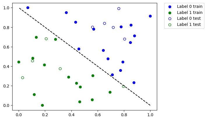
On the plot above we see:

• Solid blue dots are the samples from the training dataset labeled as 0

• Empty blue dots are the samples from the test dataset labeled as 0

• Solid green dots are the samples from the training dataset labeled as 1

• Empty green dots are the samples from the test dataset labeled as 1

We’ll train our model using solid dots and verify it using empty dots.

2. Train a model and save it

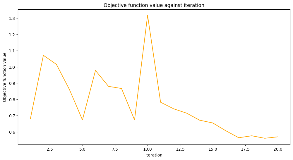
We’ll train our model in two steps. On the first step we train our model in 20 iterations.

maxiter = 20

Create an empty array for callback to store values of the objective function.

objective_values = []

We re-use a callback function from the Neural Network Classifier & Regressor tutorial to plot iteration versus objective function value with some minor tweaks to plot objective values at each step.

# callback function that draws a live plot when the .fit() method is called
def callback_graph(_, objective_value):
    clear_output(wait=True)
    objective_values.append(objective_value)

    plt.title("Objective function value against iteration")
    plt.xlabel("Iteration")
    plt.ylabel("Objective function value")

    stage1_len = np.min((len(objective_values), maxiter))
    stage1_x = np.linspace(1, stage1_len, stage1_len)
    stage1_y = objective_values[:stage1_len]

    stage2_len = np.max((0, len(objective_values) - maxiter))
    stage2_x = np.linspace(maxiter, maxiter + stage2_len - 1, stage2_len)
    stage2_y = objective_values[maxiter : maxiter + stage2_len]

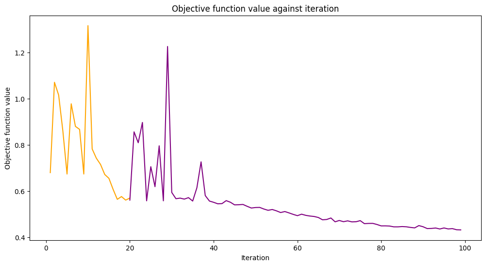
    plt.plot(stage1_x, stage1_y, color="orange")
    plt.plot(stage2_x, stage2_y, color="purple")
    plt.show()


plt.rcParams["figure.figsize"] = (12, 6)

As mentioned above we train a VQC model and set COBYLA as an optimizer with a chosen value of the maxiter parameter. Then we evaluate performance of the model to see how well it was trained. Then we save this model for a file. On the second step we load this model and will continue to work with it.

Here, we manually construct an ansatz to fix an initial point where to start optimization from.

original_optimizer = COBYLA(maxiter=maxiter)

ansatz = RealAmplitudes(num_features)
initial_point = np.asarray([0.5] * ansatz.num_parameters)

We create a model and set a sampler to the first sampler we created earlier.

original_classifier = VQC(
    ansatz=ansatz, optimizer=original_optimizer, callback=callback_graph, sampler=sampler1
)

Now it is time to train the model.

original_classifier.fit(train_features, train_labels)

<qiskit_machine_learning.algorithms.classifiers.vqc.VQC at 0x7fb74126db20>

Let’s see how well our model performs after the first step of training.

print("Train score", original_classifier.score(train_features, train_labels))
print("Test score ", original_classifier.score(test_features, test_labels))

Train score 0.8333333333333334
Test score  0.8

Next, we save the model. You may choose any file name you want. Please note that the save method does not append an extension if it is not specified in the file name.

original_classifier.save("vqc_classifier.model")

3. Load a model and continue training

To load a model a user have to call a class method load of the corresponding model class. In our case it is VQC. We pass the same file name we used in the previous section where we saved our model.

loaded_classifier = VQC.load("vqc_classifier.model")

Next, we want to alter the model in a way it can be trained further and on another simulator. To do so, we set the warm_start property. When it is set to True and fit() is called again the model uses weights from previous fit to start a new fit. We also set the sampler property of the underlying network to the second instance of the Sampler primitive we created in the beginning of the tutorial. Finally, we create and set a new optimizer with maxiter is set to 80, so the total number of iterations is 100.

loaded_classifier.warm_start = True
loaded_classifier.neural_network.sampler = sampler2
loaded_classifier.optimizer = COBYLA(maxiter=80)

Now we continue training our model from the state we finished in the previous section.

loaded_classifier.fit(train_features, train_labels)

<qiskit_machine_learning.algorithms.classifiers.vqc.VQC at 0x7fb7411cb760>

print("Train score", loaded_classifier.score(train_features, train_labels))
print("Test score", loaded_classifier.score(test_features, test_labels))

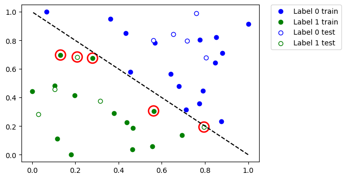
Train score 0.9
Test score 0.8

Let’s see which data points were misclassified. First, we call predict to infer predicted values from the training and test features.

train_predicts = loaded_classifier.predict(train_features)
test_predicts = loaded_classifier.predict(test_features)

Plot the whole dataset and the highlight the points that were classified incorrectly.

# return plot to default figsize
plt.rcParams["figure.figsize"] = (6, 4)

plot_dataset()

# plot misclassified data points
plt.scatter(
    train_features[np.all(train_labels != train_predicts, axis=1), 0],
    train_features[np.all(train_labels != train_predicts, axis=1), 1],
    s=200,
    facecolors="none",
    edgecolors="r",
    linewidths=2,
)
plt.scatter(
    test_features[np.all(test_labels != test_predicts, axis=1), 0],
    test_features[np.all(test_labels != test_predicts, axis=1), 1],
    s=200,
    facecolors="none",
    edgecolors="r",
    linewidths=2,
)

<matplotlib.collections.PathCollection at 0x7fb6e04c2eb0>

So, if you have a large dataset or a large model you can train it in multiple steps as shown in this tutorial.

4. PyTorch hybrid models

To save and load hybrid models, when using the TorchConnector, follow the PyTorch recommendations of saving and loading the models. For more details please refer to the PyTorch Connector tutorial where a short snippet shows how to do it.

Take a look at this pseudo-like code to get the idea:

# create a QNN and a hybrid model
qnn = create_qnn()
model = Net(qnn)
# ... train the model ...

# save the model
torch.save(model.state_dict(), "model.pt")

# create a new model
new_qnn = create_qnn()
loaded_model = Net(new_qnn)
loaded_model.load_state_dict(torch.load("model.pt"))

import qiskit.tools.jupyter

%qiskit_version_table
%qiskit_copyright

Version Information

Qiskit Software	Version
qiskit-terra	0.25.0
qiskit-aer	0.13.0
qiskit-machine-learning	0.7.0
System information
Python version	3.8.13
Python compiler	Clang 12.0.0
Python build	default, Oct 19 2022 17:54:22
OS	Darwin
CPUs	10
Memory (Gb)	64.0
Mon Jun 12 11:51:03 2023 IST

This code is a part of Qiskit

© Copyright IBM 2017, 2023.

This code is licensed under the Apache License, Version 2.0. You may
obtain a copy of this license in the LICENSE.txt file in the root directory
of this source tree or at http://www.apache.org/licenses/LICENSE-2.0.

Any modifications or derivative works of this code must retain this
copyright notice, and modified files need to carry a notice indicating
that they have been altered from the originals.