Примечание
Страница создана на основе docs/tutorials/05_torch_connector.ipynb.
Torch Connector и гибридные QNN#
This tutorial introduces the TorchConnector class, and demonstrates how it allows for a natural integration of any NeuralNetwork from Qiskit Machine Learning into a PyTorch workflow. TorchConnector takes a NeuralNetwork and makes it available as a PyTorch Module. The resulting module can be seamlessly incorporated into PyTorch classical architectures and trained jointly without additional considerations, enabling the development and testing of novel hybrid
quantum-classical machine learning architectures.
Содержание:#
Часть 1: Простая классификация и регрессия
The first part of this tutorial shows how quantum neural networks can be trained using PyTorch’s automatic differentiation engine (torch.autograd, link) for simple classification and regression tasks.
Классификация
Classification with PyTorch and
EstimatorQNNClassification with PyTorch and
SamplerQNN
Регрессия
Regression with PyTorch and
EstimatorQNN
Часть 2: Классификация MNIST, гибридные QNNs
Вторая часть этого урока показывает, как встроить (квантовую) NeuralNetwork в целевой рабочий процесс PyTorch (в данном случае, типичную архитектуру CNN) для классификации данных MNIST гибридным квантово-классическим способом.
[1]:
# Necessary imports

import numpy as np
import matplotlib.pyplot as plt

from torch import Tensor
from torch.nn import Linear, CrossEntropyLoss, MSELoss
from torch.optim import LBFGS

from qiskit import QuantumCircuit
from qiskit.circuit import Parameter
from qiskit.circuit.library import RealAmplitudes, ZZFeatureMap
from qiskit_algorithms.utils import algorithm_globals
from qiskit_machine_learning.neural_networks import SamplerQNN, EstimatorQNN
from qiskit_machine_learning.connectors import TorchConnector

# Set seed for random generators
algorithm_globals.random_seed = 42
Часть 1: Простая классификация и регрессия#
1. Классификация#
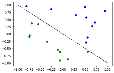
First, we show how TorchConnector allows to train a Quantum NeuralNetwork to solve a classification tasks using PyTorch’s automatic differentiation engine. In order to illustrate this, we will perform binary classification on a randomly generated dataset.
[2]:
# Generate random dataset

# Select dataset dimension (num_inputs) and size (num_samples)
num_inputs = 2
num_samples = 20

# Generate random input coordinates (X) and binary labels (y)
X = 2 * algorithm_globals.random.random([num_samples, num_inputs]) - 1
y01 = 1 * (np.sum(X, axis=1) >= 0)  # in { 0,  1}, y01 will be used for SamplerQNN example
y = 2 * y01 - 1  # in {-1, +1}, y will be used for EstimatorQNN example

# Convert to torch Tensors
X_ = Tensor(X)
y01_ = Tensor(y01).reshape(len(y)).long()
y_ = Tensor(y).reshape(len(y), 1)

# Plot dataset
for x, y_target in zip(X, y):
    if y_target == 1:
        plt.plot(x[0], x[1], "bo")
    else:
        plt.plot(x[0], x[1], "go")
plt.plot([-1, 1], [1, -1], "--", color="black")
plt.show()
A. Classification with PyTorch and EstimatorQNN#
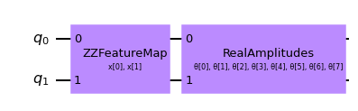
Linking an EstimatorQNN to PyTorch is relatively straightforward. Here we illustrate this by using the EstimatorQNN constructed from a feature map and an ansatz.
[3]:
# Set up a circuit
feature_map = ZZFeatureMap(num_inputs)
ansatz = RealAmplitudes(num_inputs)
qc = QuantumCircuit(num_inputs)
qc.compose(feature_map, inplace=True)
qc.compose(ansatz, inplace=True)
qc.draw("mpl")
[3]:
[4]:
# Setup QNN
qnn1 = EstimatorQNN(
    circuit=qc, input_params=feature_map.parameters, weight_params=ansatz.parameters
)

# Set up PyTorch module
# Note: If we don't explicitly declare the initial weights
# they are chosen uniformly at random from [-1, 1].
initial_weights = 0.1 * (2 * algorithm_globals.random.random(qnn1.num_weights) - 1)
model1 = TorchConnector(qnn1, initial_weights=initial_weights)
print("Initial weights: ", initial_weights)
Initial weights:  [-0.01256962  0.06653564  0.04005302 -0.03752667  0.06645196  0.06095287
 -0.02250432 -0.04233438]
[5]:
# Test with a single input
model1(X_[0, :])
[5]:
tensor([-0.3285], grad_fn=<_TorchNNFunctionBackward>)
Оптимизатор#
The choice of optimizer for training any machine learning model can be crucial in determining the success of our training’s outcome. When using TorchConnector, we get access to all of the optimizer algorithms defined in the [torch.optim] package (link). Some of the most famous algorithms used in popular machine learning architectures include Adam, SGD, or Adagrad. However, for this tutorial we will be using the L-BFGS algorithm
(torch.optim.LBFGS), one of the most well know second-order optimization algorithms for numerical optimization.
Функция потерь#
As for the loss function, we can also take advantage of PyTorch’s pre-defined modules from torch.nn, such as the Cross-Entropy or Mean Squared Error losses.
💡 Clarification : In classical machine learning, the general rule of thumb is to apply a Cross-Entropy loss to classification tasks, and MSE loss to regression tasks. However, this recommendation is given under the assumption that the output of the classification network is a class probability value in the \([0, 1]\) range (usually this is achieved through a Softmax layer). Because the following example for EstimatorQNN does not include such layer, and we don’t apply any mapping to
the output (the following section shows an example of application of parity mapping with SamplerQNNs), the QNN’s output can take any value in the range \([-1, 1]\). In case you were wondering, this is the reason why this particular example uses MSELoss for classification despite it not being the norm (but we encourage you to experiment with different loss functions and see how they can impact training results).
[6]:
# Define optimizer and loss
optimizer = LBFGS(model1.parameters())
f_loss = MSELoss(reduction="sum")

# Start training
model1.train()  # set model to training mode


# Note from (https://pytorch.org/docs/stable/optim.html):
# Some optimization algorithms such as LBFGS need to
# reevaluate the function multiple times, so you have to
# pass in a closure that allows them to recompute your model.
# The closure should clear the gradients, compute the loss,
# and return it.
def closure():
    optimizer.zero_grad()  # Initialize/clear gradients
    loss = f_loss(model1(X_), y_)  # Evaluate loss function
    loss.backward()  # Backward pass
    print(loss.item())  # Print loss
    return loss


# Run optimizer step4
optimizer.step(closure)
25.535646438598633
22.696760177612305
20.039228439331055
19.687908172607422
19.267208099365234
19.025373458862305
18.154708862304688
17.337854385375977
19.082578659057617
17.073287963867188
16.21839141845703
14.992582321166992
14.929339408874512
14.914533615112305
14.907636642456055
14.902364730834961
14.902134895324707
14.90211009979248
14.902111053466797
[6]:
tensor(25.5356, grad_fn=<MseLossBackward0>)
[7]:
# Evaluate model and compute accuracy
model1.eval()
y_predict = []
for x, y_target in zip(X, y):
    output = model1(Tensor(x))
    y_predict += [np.sign(output.detach().numpy())[0]]

print("Accuracy:", sum(y_predict == y) / len(y))

# Plot results
# red == wrongly classified
for x, y_target, y_p in zip(X, y, y_predict):
    if y_target == 1:
        plt.plot(x[0], x[1], "bo")
    else:
        plt.plot(x[0], x[1], "go")
    if y_target != y_p:
        plt.scatter(x[0], x[1], s=200, facecolors="none", edgecolors="r", linewidths=2)
plt.plot([-1, 1], [1, -1], "--", color="black")
plt.show()
Accuracy: 0.8
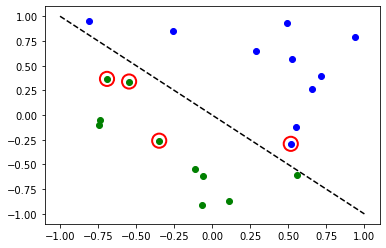
Красными кружками отмечены неверно классифицированные данные.
B. Classification with PyTorch and SamplerQNN#
Linking a SamplerQNN to PyTorch requires a bit more attention than EstimatorQNN. Without the correct setup, backpropagation is not possible.
In particular, we must make sure that we are returning a dense array of probabilities in the network’s forward pass (sparse=False). This parameter is set up to False by default, so we just have to make sure that it has not been changed.
⚠️ Attention: If we define a custom interpret function ( in the example: parity), we must remember to explicitly provide the desired output shape ( in the example: 2). For more info on the initial parameter setup for SamplerQNN, please check out the official qiskit documentation.
[8]:
# Define feature map and ansatz
feature_map = ZZFeatureMap(num_inputs)
ansatz = RealAmplitudes(num_inputs, entanglement="linear", reps=1)

# Define quantum circuit of num_qubits = input dim
# Append feature map and ansatz
qc = QuantumCircuit(num_inputs)
qc.compose(feature_map, inplace=True)
qc.compose(ansatz, inplace=True)

# Define SamplerQNN and initial setup
parity = lambda x: "{:b}".format(x).count("1") % 2  # optional interpret function
output_shape = 2  # parity = 0, 1
qnn2 = SamplerQNN(
    circuit=qc,
    input_params=feature_map.parameters,
    weight_params=ansatz.parameters,
    interpret=parity,
    output_shape=output_shape,
)

# Set up PyTorch module
# Reminder: If we don't explicitly declare the initial weights
# they are chosen uniformly at random from [-1, 1].
initial_weights = 0.1 * (2 * algorithm_globals.random.random(qnn2.num_weights) - 1)
print("Initial weights: ", initial_weights)
model2 = TorchConnector(qnn2, initial_weights)
Initial weights: [ 0.0364991 -0.0720495 -0.06001836 -0.09852755]
Для выбора оптимизатора и функции потерь вы можете вернуться к этому разделу.
[9]:
# Define model, optimizer, and loss
optimizer = LBFGS(model2.parameters())
f_loss = CrossEntropyLoss()  # Our output will be in the [0,1] range

# Start training
model2.train()

# Define LBFGS closure method (explained in previous section)
def closure():
    optimizer.zero_grad(set_to_none=True)  # Initialize gradient
    loss = f_loss(model2(X_), y01_)  # Calculate loss
    loss.backward()  # Backward pass

    print(loss.item())  # Print loss
    return loss


# Run optimizer (LBFGS requires closure)
optimizer.step(closure);
0.6925069093704224
0.6881508231163025
0.6516683101654053
0.6485998034477234
0.6394743919372559
0.7057444453239441
0.669085681438446
0.766187310218811
0.7188469171524048
0.7919709086418152
0.7598814964294434
0.7028256058692932
0.7486447095870972
0.6890242695808411
0.7760348916053772
0.7892935276031494
0.7556288242340088
0.7058126330375671
0.7203161716461182
0.7030722498893738
[10]:
# Evaluate model and compute accuracy
model2.eval()
y_predict = []
for x in X:
    output = model2(Tensor(x))
    y_predict += [np.argmax(output.detach().numpy())]

print("Accuracy:", sum(y_predict == y01) / len(y01))

# plot results
# red == wrongly classified
for x, y_target, y_ in zip(X, y01, y_predict):
    if y_target == 1:
        plt.plot(x[0], x[1], "bo")
    else:
        plt.plot(x[0], x[1], "go")
    if y_target != y_:
        plt.scatter(x[0], x[1], s=200, facecolors="none", edgecolors="r", linewidths=2)
plt.plot([-1, 1], [1, -1], "--", color="black")
plt.show()
Accuracy: 0.5
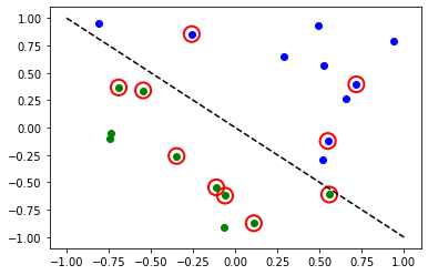
Красными кружками отмечены неверно классифицированные данные.
2. Регрессия#
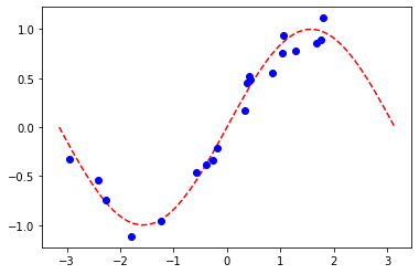
We use a model based on the EstimatorQNN to also illustrate how to perform a regression task. The chosen dataset in this case is randomly generated following a sine wave.
[11]:
# Generate random dataset

num_samples = 20
eps = 0.2
lb, ub = -np.pi, np.pi
f = lambda x: np.sin(x)

X = (ub - lb) * algorithm_globals.random.random([num_samples, 1]) + lb
y = f(X) + eps * (2 * algorithm_globals.random.random([num_samples, 1]) - 1)
plt.plot(np.linspace(lb, ub), f(np.linspace(lb, ub)), "r--")
plt.plot(X, y, "bo")
plt.show()
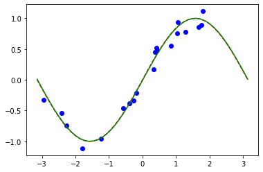
A. Regression with PyTorch and EstimatorQNN#
The network definition and training loop will be analogous to those of the classification task using EstimatorQNN. In this case, we define our own feature map and ansatz, but let’s do it a little different.
[12]:
# Construct simple feature map
param_x = Parameter("x")
feature_map = QuantumCircuit(1, name="fm")
feature_map.ry(param_x, 0)

# Construct simple parameterized ansatz
param_y = Parameter("y")
ansatz = QuantumCircuit(1, name="vf")
ansatz.ry(param_y, 0)

qc = QuantumCircuit(1)
qc.compose(feature_map, inplace=True)
qc.compose(ansatz, inplace=True)

# Construct QNN
qnn3 = EstimatorQNN(circuit=qc, input_params=[param_x], weight_params=[param_y])

# Set up PyTorch module
# Reminder: If we don't explicitly declare the initial weights
# they are chosen uniformly at random from [-1, 1].
initial_weights = 0.1 * (2 * algorithm_globals.random.random(qnn3.num_weights) - 1)
model3 = TorchConnector(qnn3, initial_weights)
Для выбора оптимизатора и функции потерь вы можете вернуться к этому разделу.
[13]:
# Define optimizer and loss function
optimizer = LBFGS(model3.parameters())
f_loss = MSELoss(reduction="sum")

# Start training
model3.train()  # set model to training mode

# Define objective function
def closure():
    optimizer.zero_grad(set_to_none=True)  # Initialize gradient
    loss = f_loss(model3(Tensor(X)), Tensor(y))  # Compute batch loss
    loss.backward()  # Backward pass
    print(loss.item())  # Print loss
    return loss


# Run optimizer
optimizer.step(closure)
14.947757720947266
2.948650360107422
8.952412605285645
0.37905153632164
0.24995625019073486
0.2483610212802887
0.24835753440856934
[13]:
tensor(14.9478, grad_fn=<MseLossBackward0>)
[14]:
# Plot target function
plt.plot(np.linspace(lb, ub), f(np.linspace(lb, ub)), "r--")

# Plot data
plt.plot(X, y, "bo")

# Plot fitted line
model3.eval()
y_ = []
for x in np.linspace(lb, ub):
    output = model3(Tensor([x]))
    y_ += [output.detach().numpy()[0]]
plt.plot(np.linspace(lb, ub), y_, "g-")
plt.show()
Часть 2: Классификация MNIST, гибридные QNN#
В этой второй части мы показываем, как использовать гибридно-классическую нейронную сеть с помощью TorchConnector для выполнения более сложной задачи по классификации изображений на наборе данных с рукописными буквами MNIST.
Для более подробного (до TorchConnector) объяснения гибридных кванто-классических нейронных сетей вы можете посмотреть соответствующий раздел в Qiskit Textbook.
[15]:
# Additional torch-related imports
import torch
from torch import cat, no_grad, manual_seed
from torch.utils.data import DataLoader
from torchvision import datasets, transforms
import torch.optim as optim
from torch.nn import (
    Module,
    Conv2d,
    Linear,
    Dropout2d,
    NLLLoss,
    MaxPool2d,
    Flatten,
    Sequential,
    ReLU,
)
import torch.nn.functional as F
Шаг 1: Определение загрузчиков данных для обучения и тестирования#
Мы пользуемся преимуществом torchvision API для непосредственной загрузки подмножества набора данных MNIST и определения DataLoader (link) для обучения и тестирования.
[16]:
# Train Dataset
# -------------

# Set train shuffle seed (for reproducibility)
manual_seed(42)

batch_size = 1
n_samples = 100  # We will concentrate on the first 100 samples

# Use pre-defined torchvision function to load MNIST train data
X_train = datasets.MNIST(
    root="./data", train=True, download=True, transform=transforms.Compose([transforms.ToTensor()])
)

# Filter out labels (originally 0-9), leaving only labels 0 and 1
idx = np.append(
    np.where(X_train.targets == 0)[0][:n_samples], np.where(X_train.targets == 1)[0][:n_samples]
)
X_train.data = X_train.data[idx]
X_train.targets = X_train.targets[idx]

# Define torch dataloader with filtered data
train_loader = DataLoader(X_train, batch_size=batch_size, shuffle=True)
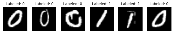
Если мы выполним быструю визуализацию, то станет видно, что набор данных для обучения состоит из изображений написанных вручную цифр 0 и 1.
[17]:
n_samples_show = 6

data_iter = iter(train_loader)
fig, axes = plt.subplots(nrows=1, ncols=n_samples_show, figsize=(10, 3))

while n_samples_show > 0:
    images, targets = data_iter.__next__()

    axes[n_samples_show - 1].imshow(images[0, 0].numpy().squeeze(), cmap="gray")
    axes[n_samples_show - 1].set_xticks([])
    axes[n_samples_show - 1].set_yticks([])
    axes[n_samples_show - 1].set_title("Labeled: {}".format(targets[0].item()))

    n_samples_show -= 1
[18]:
# Test Dataset
# -------------

# Set test shuffle seed (for reproducibility)
# manual_seed(5)

n_samples = 50

# Use pre-defined torchvision function to load MNIST test data
X_test = datasets.MNIST(
    root="./data", train=False, download=True, transform=transforms.Compose([transforms.ToTensor()])
)

# Filter out labels (originally 0-9), leaving only labels 0 and 1
idx = np.append(
    np.where(X_test.targets == 0)[0][:n_samples], np.where(X_test.targets == 1)[0][:n_samples]
)
X_test.data = X_test.data[idx]
X_test.targets = X_test.targets[idx]

# Define torch dataloader with filtered data
test_loader = DataLoader(X_test, batch_size=batch_size, shuffle=True)
Шаг 2: Определение QNN и гибридной модели#
This second step shows the power of the TorchConnector. After defining our quantum neural network layer (in this case, a EstimatorQNN), we can embed it into a layer in our torch Module by initializing a torch connector as TorchConnector(qnn).
⚠️ Внимание: Для правильного использования метода обратного распространения ошибки (backpropagation) для градиента в гибридных моделях, НЕОБХОДИМО установить начальный параметр input_gradients в значение TRUE во время инициализации qnn.
[19]:
# Define and create QNN
def create_qnn():
    feature_map = ZZFeatureMap(2)
    ansatz = RealAmplitudes(2, reps=1)
    qc = QuantumCircuit(2)
    qc.compose(feature_map, inplace=True)
    qc.compose(ansatz, inplace=True)

    # REMEMBER TO SET input_gradients=True FOR ENABLING HYBRID GRADIENT BACKPROP
    qnn = EstimatorQNN(
        circuit=qc,
        input_params=feature_map.parameters,
        weight_params=ansatz.parameters,
        input_gradients=True,
    )
    return qnn


qnn4 = create_qnn()
[20]:
# Define torch NN module


class Net(Module):
    def __init__(self, qnn):
        super().__init__()
        self.conv1 = Conv2d(1, 2, kernel_size=5)
        self.conv2 = Conv2d(2, 16, kernel_size=5)
        self.dropout = Dropout2d()
        self.fc1 = Linear(256, 64)
        self.fc2 = Linear(64, 2)  # 2-dimensional input to QNN
        self.qnn = TorchConnector(qnn)  # Apply torch connector, weights chosen
        # uniformly at random from interval [-1,1].
        self.fc3 = Linear(1, 1)  # 1-dimensional output from QNN

    def forward(self, x):
        x = F.relu(self.conv1(x))
        x = F.max_pool2d(x, 2)
        x = F.relu(self.conv2(x))
        x = F.max_pool2d(x, 2)
        x = self.dropout(x)
        x = x.view(x.shape[0], -1)
        x = F.relu(self.fc1(x))
        x = self.fc2(x)
        x = self.qnn(x)  # apply QNN
        x = self.fc3(x)
        return cat((x, 1 - x), -1)


model4 = Net(qnn4)
Шаг 3: Обучение#
[21]:
# Define model, optimizer, and loss function
optimizer = optim.Adam(model4.parameters(), lr=0.001)
loss_func = NLLLoss()

# Start training
epochs = 10  # Set number of epochs
loss_list = []  # Store loss history
model4.train()  # Set model to training mode

for epoch in range(epochs):
    total_loss = []
    for batch_idx, (data, target) in enumerate(train_loader):
        optimizer.zero_grad(set_to_none=True)  # Initialize gradient
        output = model4(data)  # Forward pass
        loss = loss_func(output, target)  # Calculate loss
        loss.backward()  # Backward pass
        optimizer.step()  # Optimize weights
        total_loss.append(loss.item())  # Store loss
    loss_list.append(sum(total_loss) / len(total_loss))
    print("Training [{:.0f}%]\tLoss: {:.4f}".format(100.0 * (epoch + 1) / epochs, loss_list[-1]))
Training [10%]  Loss: -1.1630
Training [20%]  Loss: -1.5294
Training [30%]  Loss: -1.7855
Training [40%]  Loss: -1.9863
Training [50%]  Loss: -2.2257
Training [60%]  Loss: -2.4513
Training [70%]  Loss: -2.6758
Training [80%]  Loss: -2.8832
Training [90%]  Loss: -3.1006
Training [100%] Loss: -3.3061
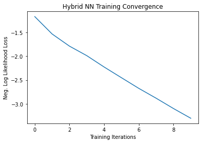
[22]:
# Plot loss convergence
plt.plot(loss_list)
plt.title("Hybrid NN Training Convergence")
plt.xlabel("Training Iterations")
plt.ylabel("Neg. Log Likelihood Loss")
plt.show()
Now we’ll save the trained model, just to show how a hybrid model can be saved and re-used later for inference. To save and load hybrid models, when using the TorchConnector, follow the PyTorch recommendations of saving and loading the models.
[23]:
torch.save(model4.state_dict(), "model4.pt")
Шаг 4: Оценка#
We start from recreating the model and loading the state from the previously saved file. You create a QNN layer using another simulator or a real hardware. So, you can train a model on real hardware available on the cloud and then for inference use a simulator or vice verse. For a sake of simplicity we create a new quantum neural network in the same way as above.
[24]:
qnn5 = create_qnn()
model5 = Net(qnn5)
model5.load_state_dict(torch.load("model4.pt"))
[24]:
<All keys matched successfully>
[25]:
model5.eval()  # set model to evaluation mode
with no_grad():

    correct = 0
    for batch_idx, (data, target) in enumerate(test_loader):
        output = model5(data)
        if len(output.shape) == 1:
            output = output.reshape(1, *output.shape)

        pred = output.argmax(dim=1, keepdim=True)
        correct += pred.eq(target.view_as(pred)).sum().item()

        loss = loss_func(output, target)
        total_loss.append(loss.item())

    print(
        "Performance on test data:\n\tLoss: {:.4f}\n\tAccuracy: {:.1f}%".format(
            sum(total_loss) / len(total_loss), correct / len(test_loader) / batch_size * 100
        )
    )
Performance on test data:
        Loss: -3.3585
        Accuracy: 100.0%
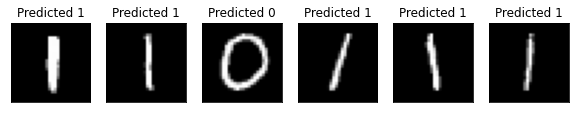
[26]:
# Plot predicted labels

n_samples_show = 6
count = 0
fig, axes = plt.subplots(nrows=1, ncols=n_samples_show, figsize=(10, 3))

model5.eval()
with no_grad():
    for batch_idx, (data, target) in enumerate(test_loader):
        if count == n_samples_show:
            break
        output = model5(data[0:1])
        if len(output.shape) == 1:
            output = output.reshape(1, *output.shape)

        pred = output.argmax(dim=1, keepdim=True)

        axes[count].imshow(data[0].numpy().squeeze(), cmap="gray")

        axes[count].set_xticks([])
        axes[count].set_yticks([])
        axes[count].set_title("Predicted {}".format(pred.item()))

        count += 1
🎉🎉🎉🎉 Теперь вы можете экспериментировать с собственными гибридными наборами данных и архитектурами, используя Qiskit Machine Learning. Удачи!
[27]:
import qiskit.tools.jupyter

%qiskit_version_table
%qiskit_copyright
Version Information
| Qiskit Software | Version |
|---|---|
qiskit-terra | 0.22.0 |
qiskit-aer | 0.11.1 |
qiskit-ignis | 0.7.0 |
qiskit | 0.33.0 |
qiskit-machine-learning | 0.5.0 |
| System information | |
| Python version | 3.7.9 |
| Python compiler | MSC v.1916 64 bit (AMD64) |
| Python build | default, Aug 31 2020 17:10:11 |
| OS | Windows |
| CPUs | 4 |
| Memory (Gb) | 31.837730407714844 |
| Thu Nov 03 09:57:38 2022 GMT Standard Time | |
This code is a part of Qiskit
© Copyright IBM 2017, 2022.
This code is licensed under the Apache License, Version 2.0. You may
obtain a copy of this license in the LICENSE.txt file in the root directory
of this source tree or at http://www.apache.org/licenses/LICENSE-2.0.
Any modifications or derivative works of this code must retain this
copyright notice, and modified files need to carry a notice indicating
that they have been altered from the originals.