참고
이 페이지는 docs/tutorials/11_quantum_convolutional_neural_networks.ipynb 에서 생성되었다.
양자 합성곱 신경망#
1. 소개#
Throughout this tutorial, we discuss a Quantum Convolutional Neural Network (QCNN), first proposed by Cong et. al. [1]. We implement such a QCNN on Qiskit by modeling both the convolutional layers and pooling layers using a quantum circuit. After building such a network, we train it to differentiate horizontal and vertical lines from a pixelated image. The following tutorial is thus divided accordingly;
QCNN과 CCNN의 차이점
QCNN의 구성 요소
데이터 생성
QCNN 구축
QCNN 학습
QCNN 테스트
참고문헌
먼저 이 튜토리얼에 필요한 라이브러리와 패키지를 불러온다.
[1]:
import json
import matplotlib.pyplot as plt
import numpy as np
from IPython.display import clear_output
from qiskit import QuantumCircuit
from qiskit.circuit import ParameterVector
from qiskit.circuit.library import ZFeatureMap
from qiskit.quantum_info import SparsePauliOp
from qiskit_algorithms.optimizers import COBYLA
from qiskit_algorithms.utils import algorithm_globals
from qiskit_machine_learning.algorithms.classifiers import NeuralNetworkClassifier
from qiskit_machine_learning.neural_networks import EstimatorQNN
from sklearn.model_selection import train_test_split

algorithm_globals.random_seed = 12345
1. QCNN과 CCNN의 차이점#
1.1 고전 합성곱 신경망#
고전 합성곱 신경망(CCNN)은 입력의 특정한 특징과 패턴을 결정할 수 있는 인공 신경망의 하위 개념이다. 이 같은 이유로 이미지 인식 및 오디오 처리에 일반적으로 사용된다.
CCNN에서 사용되는 합성곱 층과 풀링 층을 이용해서 입력데이터의 특징을 추출할 수 있다.
그림 1의 CCNN 모델은 입력 이미지가 고양이 혹은 개를 포함하는지 판단하도록 학습되었다. 이를 위해 입력 이미지는 일련의 합성곱 층(C)과 풀링 층(P)을 교대로 통과한하고, 모든 층에서 패턴을 감지되고 각 패턴이 고양이 또는 개와 연결한다. 전결합 층(FC)은 입력 이미지가 고양이인지 개인지를 결정할 수 있는 출력을 제공한다.
합성곱 층은 특정 입력의 특징 및 패턴을 판단할 수 있는 커널을 사용한다. 이것의 예는 이미지에서의 특징 검출이며, 여기서 각각의 층들은 입력 이미지 내의 특정 패턴들을 검출한다. 이는 \(ij\) 평면을 따라 특징 및 패턴을 인식하는 \(l^{th}\) 층이 있는 그림 1에 도시되어 있다. 그런 다음 이러한 특징을 학습 과정에서 주어진 출력과 연관시킬 수 있으며, 이러한 과정을 통해 데이터셋을 학습할 수 있다.
한편, 풀링 층은 입력 데이터의 차원수를 감소시키고, CCNN 에서 학습 매개변수의 양과 연산 비용을 감소시킨다. CCNN의 개략도는 아래에서 볼 수 있다.
CCNN에 대한 추가 정보는 [2]를 참조하십시오.
 Figure 1. CCNN을 사용하여 고양이와 개의 이미지를 분류하는 개략적인 시연이다. 풀링 층의 사용으로 인해 차원수가 감소하는 여러 합성곱 층과 풀링 층이 적용되는 것을 볼 수 있다. CCNN의 출력을 통해 입력 이미지가 고양이인지 개인지를 결정한다. [1] 에서 가져온 이미지이다.
1.2 양자 합성곱 신경망#
Quantum Convolutional Neural Networks (QCNN) behave in a similar manner to CCNNs. First, we encode our pixelated image into a quantum circuit using a given feature map, such Qiskit’s ZFeatureMap or ZZFeatureMap or others available in the circuit library.
이미지를 인코딩한 후 다음 섹션에서 정의된 대로 합성곱 층과 풀링 층을 교대로 적용한다. 이러한 층들을 교대로 적용함으로써, 회로의 차원을 큐비트가 한개만 남을 때까지 감소시킨다. 그런 다음 이 남은 큐비트의 출력을 측정하여 입력 이미지를 분류할 수 있다.
양자 합성곱 층은 회로의 큐비트 간의 관계를 인식하고 결정하는 두 개의 큐비트 유니타리 연산자로 구성된다. 이 유니타리 게이트는 다음 섹션에서 아래에 정의된다.
For the Quantum Pooling Layer, we cannot do the same as is done classically to reduce the dimension, i.e. the number of qubits in our circuit. Instead, we reduce the number of qubits by performing operations upon each until a specific point and then disregard certain qubits in a specific layer. It is these layers where we stop performing operations on certain qubits that we call our ‘pooling layer’. Details of the pooling layer is discussed further in the next section.
QCNN에서 각 층은 매개 변수화된 회로를 포함하며, 각 층의 매개 변수를 조정하여 출력 결과를 변경한다는 것을 의미한다. QCNN을 학습할 때 이러한 매개 변수는 QCNN의 손실 함수를 줄이기 위해 조정된다.
4개의 큐비트 QCNN의 간단한 예는 아래에서 볼 수 있다.

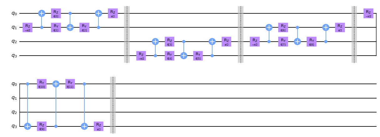
그림 2: 4개의 큐비트를 포함하는 QCNN의 예시. 첫 번째 합성곱 층은 모든 큐비트에 작용한다. 이는 첫 번째 풀링 층에 이어 첫 번째 두 개를 무시하여 QCNN의 차원수를 4개의 큐비트에서 2개의 큐비트로 감소시킨다. 그런 다음 두 번째 합성곱 층 QCNN에서 여전히 사용 중인 두 큐비트 사이의 특징을 감지하고 이어서 다른 풀링 층을 감지하여 2개의 큐비트에서 출력 큐비트가 되는 1개의 큐비트로 차원수를 감소시킨다.
2. QCNN의 구성요소#
이 튜토리얼의 섹션 1에서 논의한 바와 같이, CCNN은 합성곱 층과 풀링 층을 모두 포함할 것이다. 여기서, 양자 회로에 적용되는 게이트의 관점에서 QCNN에 대한 이러한 층을 정의하고 4개의 큐비트에 대한 각 층의 예를 보여준다.
이러한 각 층에는 손실 함수를 최소화하고 QCNN이 수평선과 수직선 사이를 분류하도록 학습하기 위해 학습 과정 전반에 걸쳐 조정된 매개 변수가 포함된다.
이론적으로, 네트워크의 합성곱 층과 풀링 층 모두에 매개 변수화된 회로를 적용할 수 있다. 예를 들어 [2] 에서 (파울리 행렬의 3차원 일반화인) Gellmann 행렬은 한 쌍의 큐비트에 작용하는 각 유니타리 게이트의 생성기로 사용된다.
여기서, 다른 접근법을 취하고 [3] 에서 제안된 것처럼 두 개의 큐비트 유니타리를 기반으로 매개 변수화된 회로를 형성한다. 이것은 \(U(4)\) 의 모든 유니타리 행렬이 다음과 같이 분해될 수 있음을 나타낸다.
여기서 \(A_j \in \text{SU}(2)\) 이고, \(\otimes\) 는 텐서 곱이며 \(N(\alpha, \beta, \gamma) = exp(i[\alpha \sigma_x\sigma_x + \beta \sigma_y\sigma_y + \gamma \sigma_z\sigma_z ])\) 에서의 \(\alpha, \beta, \gamma\) 는 조절할 수 있는 매개 변수이다.
이로부터, 각 유니타리는 15개의 매개 변수에 의존한다는 것이 분명하며, QCNN이 전체 힐베르트 공간을 포괄할 수 있으려면 QCNN의 각 유니타리가 각각 15개의 매개 변수를 포함해야 한다는 것을 암시한다.
이렇게 많은 양의 매개변수를 조정하는 것은 어렵고 긴 학습 시간이 필요할 것이다. 이 문제를 극복하기 위해, ansatz를 힐베르트 공간의 특정 하위 공간으로 제한하고 2 큐비트 유니타리 게이트를 \(N(\alpha, \beta, \gamma)\) 로 정의한다. [3] 에서 볼 수 있는 이 2 큐비트 유니타리들은 아래에서 볼 수 있으며 QCNN의 각 층에 대한 모든 인접 큐비트에 적용된다.
\(N(\alpha, \beta, \gamma)\) 를 매개 변수화된 층에 대한 2 큐비트 유니타리로만 사용함으로써, QCNN을 최적의 솔루션이 포함되지 않을 수 있는 특정 하위 공간으로 제한하고 QCNN의 정확도를 감소시킨다는 점에 유의한다. 이 튜토리얼의 의도대로 이 매개 변수화된 회로를 사용하여 QCNN의 학습 시간을 단축할 것이다.

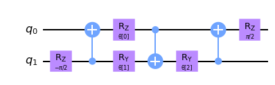
그림 3: [3] 에서 보는 바와 같이 \(N(\alpha, \beta, \gamma) = exp(i[\alpha \sigma_x\sigma_x + \beta \sigma_y\sigma_y + \gamma \sigma_z\sigma_z ])\) 에 대한 2 큐비트 유니타리 회로를 매개 변수화하였으며, 여기서 \(\alpha = \frac{\pi}{2} - 2\theta\), \(\beta = 2\phi - \frac{\pi}{2}\), \(\gamma = \frac{\pi}{2} - 2\lambda\) 는 회로에서 보는 바와 같다. 이러한 2 큐비트 유니타리는 특징 지도의 모든 인접한 큐비트에 적용할 것이다.
2.1 합성곱 층#
이 튜토리얼의 다음 단계는 QCNN의 합성곱 층을 정의한다. 이러한 층은 특징 지도를 사용하여 데이터를 인코딩한 후 큐비트에 적용된다.
먼저 합성곱 및 풀링 층을 만드는 데 사용될 매개 변수화된 유니타리 게이트를 결정해야 한다.
[2]:
# We now define a two qubit unitary as defined in [3]
def conv_circuit(params):
    target = QuantumCircuit(2)
    target.rz(-np.pi / 2, 1)
    target.cx(1, 0)
    target.rz(params[0], 0)
    target.ry(params[1], 1)
    target.cx(0, 1)
    target.ry(params[2], 1)
    target.cx(1, 0)
    target.rz(np.pi / 2, 0)
    return target


# Let's draw this circuit and see what it looks like
params = ParameterVector("θ", length=3)
circuit = conv_circuit(params)
circuit.draw("mpl", style="clifford")
[2]:
유니타리를 정의했으므로 QCNN에서 합성곱 층에 대한 함수를 생성해야 한다. 아래 conv_layer 함수에 표시된 것처럼 두 개의 큐비트 유니타리를 인접한 큐비트에 적용한다.
Note that we first apply the two qubit unitary to all even pairs of qubits followed by applying to odd pairs of qubits in a circular coupling manner, i.e. the as well as neighboring qubits being coupled, the first and final qubit are also coupled through a unitary gate.
그래프를 그릴때 편의를 위해 양자 회로에 배리어를 추가하지만 실제 QCNN에는 필요하지 않으며 다음 회로에서 추출할 수 있다.
[3]:
def conv_layer(num_qubits, param_prefix):
    qc = QuantumCircuit(num_qubits, name="Convolutional Layer")
    qubits = list(range(num_qubits))
    param_index = 0
    params = ParameterVector(param_prefix, length=num_qubits * 3)
    for q1, q2 in zip(qubits[0::2], qubits[1::2]):
        qc = qc.compose(conv_circuit(params[param_index : (param_index + 3)]), [q1, q2])
        qc.barrier()
        param_index += 3
    for q1, q2 in zip(qubits[1::2], qubits[2::2] + [0]):
        qc = qc.compose(conv_circuit(params[param_index : (param_index + 3)]), [q1, q2])
        qc.barrier()
        param_index += 3

    qc_inst = qc.to_instruction()

    qc = QuantumCircuit(num_qubits)
    qc.append(qc_inst, qubits)
    return qc


circuit = conv_layer(4, "θ")
circuit.decompose().draw("mpl", style="clifford")
[3]:
2.2 풀링 층#
The purpose of a pooling layer is to reduce the dimensions of our Quantum Circuit, i.e. reduce the number of qubits in our circuit, while retaining as much information as possible from previously learned data. Reducing the amount of qubits also reduces the computational cost of the overall circuit, as the number of parameters that the QCNN needs to learn decreases.
그러나 양자 회로의 큐비트의 양을 단순히 줄일 수는 없다. 이 때문에 풀링 층을 기존의 접근 방식과 다른 방식으로 정의해야 한다.
To ‘artificially’ reduce the number of qubits in our circuit, we first begin by creating pairs of the \(N\) qubits in our system.
처음에 모든 큐비트를 쌍으로 구성한 후 앞에서 설명한 것처럼 일반화된 2 큐비트 유니타리를 각 쌍에 적용한다. 이 2 큐비트 유니타리를 적용한 후, 신경망의 나머지 부분에는 각 큐비트 쌍마다 하나의 큐비트를 무시한다.
This layer therefore has the overall effect of ‘combining’ the information of the two qubits into one qubit by first applying the unitary circuit, encoding information from one qubit into another, before disregarding one of qubits for the remainder of the circuit and not performing any operations or measurements on it.
풀링 층에서 차원수를 줄이기 위해 동적 회로를 적용할 수도 있다. 회로의 특정 큐비트에 대한 측정을 수행하고 풀링 층에서 중간의 고전적 피드백 루프를 갖는 것을 포함한다. 이러한 측정을 적용함으로써 회로의 차원수도 줄일 수 있다.
이 튜토리얼에서는 이전 접근 방식을 적용하고 각 풀링 층의 큐비트를 무시한다. 따라서 이 접근 방식을 사용하여 \(N\) 큐비트 양자 회로의 차원수를 \(N/2\) 로 변환하는 QCNN 풀링 층을 만든다.
이를 위해 먼저 2 큐비트 시스템을 하나로 변환하는 2 큐비트 유니타리를 정의한다.
[4]:
def pool_circuit(params):
    target = QuantumCircuit(2)
    target.rz(-np.pi / 2, 1)
    target.cx(1, 0)
    target.rz(params[0], 0)
    target.ry(params[1], 1)
    target.cx(0, 1)
    target.ry(params[2], 1)

    return target


params = ParameterVector("θ", length=3)
circuit = pool_circuit(params)
circuit.draw("mpl", style="clifford")
[4]:
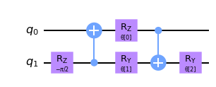
이 2 큐비트 유니타리 회로를 적용한 후, 다음층에서 첫 번째 큐비트(q0)를 무시하고 QCNN에서 두 번째 큐비트(q1)만 사용한다.
2 큐비트 풀링 층을 다른 큐비트 쌍에 적용하여 N 큐비트에 대한 풀링 층을 생성한다. 4개의 큐비트에 대해 그래프를 그려 예를 들어보겠다.
[5]:
def pool_layer(sources, sinks, param_prefix):
    num_qubits = len(sources) + len(sinks)
    qc = QuantumCircuit(num_qubits, name="Pooling Layer")
    param_index = 0
    params = ParameterVector(param_prefix, length=num_qubits // 2 * 3)
    for source, sink in zip(sources, sinks):
        qc = qc.compose(pool_circuit(params[param_index : (param_index + 3)]), [source, sink])
        qc.barrier()
        param_index += 3

    qc_inst = qc.to_instruction()

    qc = QuantumCircuit(num_qubits)
    qc.append(qc_inst, range(num_qubits))
    return qc


sources = [0, 1]
sinks = [2, 3]
circuit = pool_layer(sources, sinks, "θ")
circuit.decompose().draw("mpl", style="clifford")
[5]:
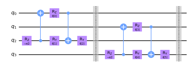
In this particular example, we reduce the dimensionality of our four qubit circuit to the last two qubits, i.e. the last two qubits in this particular example. These qubits are then used in the next layer, while the first two are neglected for the remainder of the QCNN.
3. 데이터 생성#
CCNN의 일반적인 용도는 이미지 분류기로, CCNN은 합성곱 층에서 특징 지도를 사용하여 픽셀화된 이미지의 (직선 또는 곡선 등)특정 특징과 패턴을 감지한다. 이러한 특징간의 관계를 학습함으로써 손으로 쓴 숫자를 쉽게 분류하고 라벨을 지정 할 수 있다.
Because of a classical CNN’s ability to recognize features and patterns easily, we will train our QCNN to also determine patterns and features of a given set of pixelated images, and classify between two different patterns.
데이터셋을 단순화하기 위해 2 x 4 픽셀 이미지만 고려한다. QCNN을 학습하여 구별하는 패턴은 노이즈가 많은 배경과 동시에 이미지 어디에나 놓일 수 있는 수평 또는 수직선이 될 것이다.
We first begin by generating this dataset. To create a ‘horizontal’ or ‘vertical’ line, we assign pixels value to be \(\frac{\pi}{2}\) which will represent the line in our pixelated image. We create a noisy background by assigning every other pixel a random value between \(0\) and \(\frac{\pi}{4}\) which will create a noisy background.
데이터셋을 만들 때 신경망을 각각 훈련하고 테스트하는 데이터셋인 학습 세트와 테스트 이미지 세트로 분할해야 한다.
또한 QCNN이 두 패턴을 구별하는 방법을 배울 수 있도록 데이터셋에 레이블을 지정해야 한다. 이 예제에서는 이미지에서의 수평선을 -1, 이미지에서의 수직선을 +1로 레이블 하였다.
[6]:
def generate_dataset(num_images):
    images = []
    labels = []
    hor_array = np.zeros((6, 8))
    ver_array = np.zeros((4, 8))

    j = 0
    for i in range(0, 7):
        if i != 3:
            hor_array[j][i] = np.pi / 2
            hor_array[j][i + 1] = np.pi / 2
            j += 1

    j = 0
    for i in range(0, 4):
        ver_array[j][i] = np.pi / 2
        ver_array[j][i + 4] = np.pi / 2
        j += 1

    for n in range(num_images):
        rng = algorithm_globals.random.integers(0, 2)
        if rng == 0:
            labels.append(-1)
            random_image = algorithm_globals.random.integers(0, 6)
            images.append(np.array(hor_array[random_image]))
        elif rng == 1:
            labels.append(1)
            random_image = algorithm_globals.random.integers(0, 4)
            images.append(np.array(ver_array[random_image]))

        # Create noise
        for i in range(8):
            if images[-1][i] == 0:
                images[-1][i] = algorithm_globals.random.uniform(0, np.pi / 4)
    return images, labels
Let’s now create our dataset below and split it into our test and training datasets. We pass a random_state so the split will be the same each time this notebook is run so the final results do not vary.
[7]:
images, labels = generate_dataset(50)

train_images, test_images, train_labels, test_labels = train_test_split(
    images, labels, test_size=0.3, random_state=246
)
Let’s see some examples in our dataset
[8]:
fig, ax = plt.subplots(2, 2, figsize=(10, 6), subplot_kw={"xticks": [], "yticks": []})
for i in range(4):
    ax[i // 2, i % 2].imshow(
        train_images[i].reshape(2, 4),  # Change back to 2 by 4
        aspect="equal",
    )
plt.subplots_adjust(wspace=0.1, hspace=0.025)
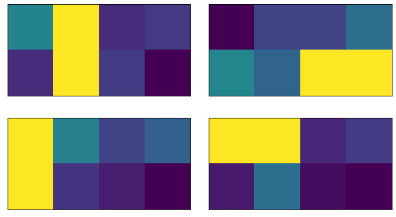
각 이미지에는 수직 또는 수평선이 포함되어 있으므로 QCNN은 구별하는 방법을 학습한다. 데이터셋을 구축했으므로 이제 QCNN의 구성 요소에 대해 논의하고 모델을 구축해보자.
4. QCNN 모델링#
이제 두 합성곱 층을 모두 정의했으므로 이제 풀링 층과 합성곱 층이 교대로 구성될 QCNN을 구축해보자.
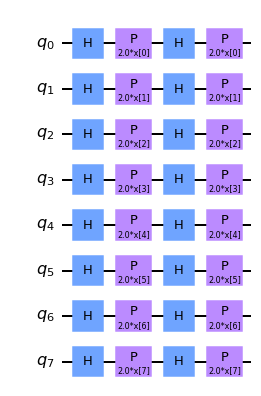
데이터셋의 이미지는 8개의 픽셀을 포함하므로 QCNN에서 8개의 큐비트를 사용한다.
We encode our dataset into our QCNN by applying a feature map. One can create a feature map using one of Qiskit’s built in feature maps, such as ZFeatureMap or ZZFeatureMap.
이 데이터셋에 대해 여러 가지 다른 기능 맵을 분석한 결과, Z 특징 지도를 사용할 때 QCNN이 가장 높은 정확도를 얻는 것으로 나타났다. 따라서 나머지 튜토리얼에서는 Z 특징 지도를 사용할 것이며 아래에서 확인할 수 있다.
[9]:
feature_map = ZFeatureMap(8)
feature_map.decompose().draw("mpl", style="clifford")
[9]:
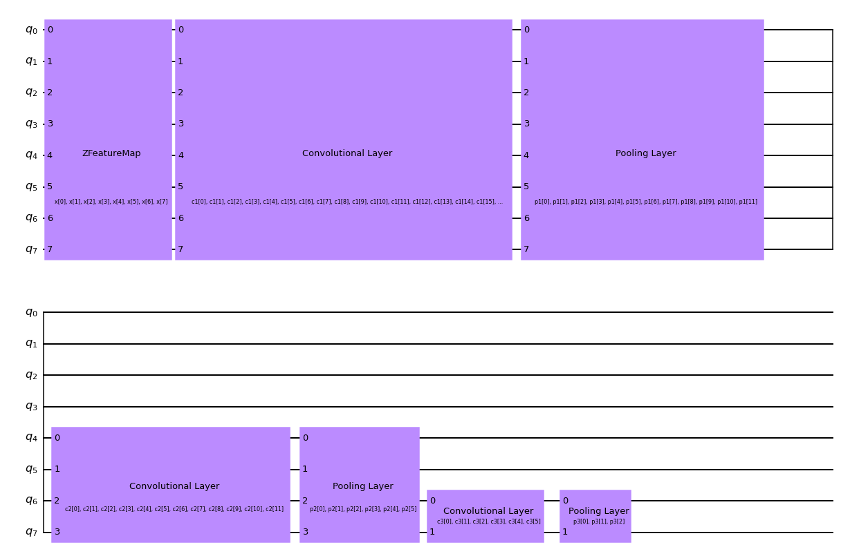
아래 개략도에서 볼 수 있는 것처럼 3개 세트의 합성곱 및 풀링 층이 교대로 배치된 QCNN에 대한 함수를 만든다. 따라서 풀링 층을 사용하여 QCNN의 차원수를 8개의 큐비트에서 1개의 큐비트로 줄인다.

수평선과 수직선의 이미지 데이터셋을 분류하기 위해 최종 큐비트의 파울리 Z 연산자의 기댓값을 측정한다. 얻어진 값이 +1 또는 -1인지에 따라 입력 이미지가 수평선 또는 수직선을 포함하였다고 결론지을 수 있다.
5. QCNN 학습#
다음 단계는 학습 데이터를 사용하여 모델을 구축하는 것이다.
시스템을 분류하기 위해 출력 회로에서 측정을 수행한다. 따라서 얻은 값은 입력 데이터에 수직선이 포함되는지 수평선이 포함되는지 여부를 분류할 것이다.
The measurement we have chosen in this tutorial is \(<Z>\), i.e. the expectation value of the Pauli Z qubit for the final qubit. Measuring this expectation value, we obtain +1 or -1, which correspond to a vertical or horizontal line respectively.
[10]:
feature_map = ZFeatureMap(8)

ansatz = QuantumCircuit(8, name="Ansatz")

# First Convolutional Layer
ansatz.compose(conv_layer(8, "c1"), list(range(8)), inplace=True)

# First Pooling Layer
ansatz.compose(pool_layer([0, 1, 2, 3], [4, 5, 6, 7], "p1"), list(range(8)), inplace=True)

# Second Convolutional Layer
ansatz.compose(conv_layer(4, "c2"), list(range(4, 8)), inplace=True)

# Second Pooling Layer
ansatz.compose(pool_layer([0, 1], [2, 3], "p2"), list(range(4, 8)), inplace=True)

# Third Convolutional Layer
ansatz.compose(conv_layer(2, "c3"), list(range(6, 8)), inplace=True)

# Third Pooling Layer
ansatz.compose(pool_layer([0], [1], "p3"), list(range(6, 8)), inplace=True)

# Combining the feature map and ansatz
circuit = QuantumCircuit(8)
circuit.compose(feature_map, range(8), inplace=True)
circuit.compose(ansatz, range(8), inplace=True)

observable = SparsePauliOp.from_list([("Z" + "I" * 7, 1)])

# we decompose the circuit for the QNN to avoid additional data copying
qnn = EstimatorQNN(
    circuit=circuit.decompose(),
    observables=observable,
    input_params=feature_map.parameters,
    weight_params=ansatz.parameters,
)
[11]:
circuit.draw("mpl", style="clifford")
[11]:
또한 모델을 학습할 때 사용할 콜백 함수를 정의한다. 이를 통해 학습 과정의 각 회차당 손실 함수를 보고 표시 할 수 있다.
[12]:
def callback_graph(weights, obj_func_eval):
    clear_output(wait=True)
    objective_func_vals.append(obj_func_eval)
    plt.title("Objective function value against iteration")
    plt.xlabel("Iteration")
    plt.ylabel("Objective function value")
    plt.plot(range(len(objective_func_vals)), objective_func_vals)
    plt.show()
이 예에서, 분류 기계 학습 알고리즘에 일반적으로 사용되는 수치 최적화 방법인 분류기를 학습하기 위해 COBYLA 최적화기를 사용한다.
We then place the the callback function, optimizer and operator of our QCNN created above into Qiskit Machine Learning’s built in Neural Network Classifier, which we can then use to train our model.
Since model training may take a long time we have already pre-trained the model for some iterations and saved the pre-trained weights. We’ll continue training from that point by setting initial_point to a vector of pre-trained weights.
[13]:
with open("11_qcnn_initial_point.json", "r") as f:
    initial_point = json.load(f)

classifier = NeuralNetworkClassifier(
    qnn,
    optimizer=COBYLA(maxiter=200),  # Set max iterations here
    callback=callback_graph,
    initial_point=initial_point,
)
After creating this classifier, we can train our QCNN using our training dataset and each image’s corresponding label. Because we previously defined the callback function, we plot the overall loss of our system per iteration.
QCNN을 학습하는 데 시간이 걸릴 수 있으므로 인내심이 필요하다.
[14]:
x = np.asarray(train_images)
y = np.asarray(train_labels)

objective_func_vals = []
plt.rcParams["figure.figsize"] = (12, 6)
classifier.fit(x, y)

# score classifier
print(f"Accuracy from the train data : {np.round(100 * classifier.score(x, y), 2)}%")
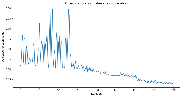
Accuracy from the train data : 97.14%
As we can see from above, the QCNN converges slowly, hence our initial_point was already close to an optimal solution. The next step is to determine whether our QCNN can classify data seen in our test image data set.
6. QCNN 테스트#
데이터셋을 구축하고 학습한 후, QCNN이 테스트 데이터셋에 없는 이미지를 예측할 수 있는지 테스트한다.
[15]:
y_predict = classifier.predict(test_images)
x = np.asarray(test_images)
y = np.asarray(test_labels)
print(f"Accuracy from the test data : {np.round(100 * classifier.score(x, y), 2)}%")

# Let's see some examples in our dataset
fig, ax = plt.subplots(2, 2, figsize=(10, 6), subplot_kw={"xticks": [], "yticks": []})
for i in range(0, 4):
    ax[i // 2, i % 2].imshow(test_images[i].reshape(2, 4), aspect="equal")
    if y_predict[i] == -1:
        ax[i // 2, i % 2].set_title("The QCNN predicts this is a Horizontal Line")
    if y_predict[i] == +1:
        ax[i // 2, i % 2].set_title("The QCNN predicts this is a Vertical Line")
plt.subplots_adjust(wspace=0.1, hspace=0.5)
Accuracy from the test data : 93.33%
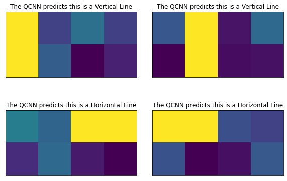
위에서 보면, QCNN이 수평선과 수직선을 분류할 수 있다는 것을 알 수 있다. 드디어 양자 회로와 양자 합성곱 및 풀링 층을 사용하여 양자 합성곱 신경망을 구축하는데 성공했다!
7. 참조#
[1] Cong, I., Choi, S. & Lukin, M.D. Quantum convolutional neural networks. Nat. Phys. 15, 1273–1278 (2019). https://doi.org/10.1038/s41567-019-0648-8
[2] IBM Convolutional Neural Networks https://www.ibm.com/cloud/learn/convolutional-neural-networks
[3] Vatan, Farrokh, and Colin Williams. “Optimal quantum circuits for general two-qubit gates.” Physical Review A 69.3 (2004): 032315.
[16]:
import qiskit.tools.jupyter

%qiskit_version_table
%qiskit_copyright
Version Information
| Software | Version |
|---|---|
qiskit | 1.0.0.dev0+737f21b |
qiskit_algorithms | 0.3.0 |
qiskit_machine_learning | 0.8.0 |
| System information | |
| Python version | 3.9.7 |
| Python compiler | GCC 7.5.0 |
| Python build | default, Sep 16 2021 13:09:58 |
| OS | Linux |
| CPUs | 2 |
| Memory (Gb) | 5.792198181152344 |
| Thu Dec 14 13:53:25 2023 EST | |
This code is a part of Qiskit
© Copyright IBM 2017, 2023.
This code is licensed under the Apache License, Version 2.0. You may
obtain a copy of this license in the LICENSE.txt file in the root directory
of this source tree or at http://www.apache.org/licenses/LICENSE-2.0.
Any modifications or derivative works of this code must retain this
copyright notice, and modified files need to carry a notice indicating
that they have been altered from the originals.