참고
이 페이지는 docs/tutorials/10_effective_dimension.ipynb 에서 생성되었다.
Qiskit Neural Networks의 유효 차원#
이 튜토리얼에서는 EffectiveDimension 및 LocalEffectiveDimension 클래스의 이점을 활용하여 양자 신경망 모델의 성능을 평가할 것이다. 이 것들은 학습 가능성, 표현 가능성 또는 일반화 능력과 같은 개념과 연결되는 정보 기하학을 기반으로 하는 메트릭이다.
코드 예제로 들어가기 전, 이 두 측정항목의 차이점과 양자 신경망 연구와 관련된 이유를 간략하게 살펴보자. 글로벌 유효 차원에 대한 자세한 내용은 본 논문 에서 확인할 수 있으며, 로컬 유효 차원은 심화 읽기 자료 에서 확인 할 수 있다.
1. Global vs. Local Effective Dimension#
Both classical and quantum machine learning models share a common goal: being good at generalizing, i.e. learning insights from data and applying them on unseen data.
이 능력을 평가하기 위한 좋은 지표를 찾는 것은 중요한 문제이다. The Power of Quantum Neural Networks 에서 저자는 글로벌(global) 유효 차원을 새로운 데이터에 대해 특정 모델이 얼마나 잘 수행할 수 있는지에 대한 유용한 지표로 소개한다. Effective Dimension of Machine Learning Models 에서는 기계 학습 모델의 일반화 오차를 제한하는 새로운 용량 척도로 로컬(local) 유효 차원이 제안되었다.
글로벌 (EffectiveDimension 클래스)과 로컬 유효 차원(LocalEffectiveDimension 클래스)의 주요 차이점은 실제로 계산되는 방식이 아니라 분석되는 매개변수 공간의 특성에 있다 . 글로벌 유효 차원은 모델의 전체 매개변수 공간 을 통합하며 많은 수의 매개변수(가중치) 세트 에서 된다. 반면에 로컬 유효 차원은 훈련된 모델이 새 데이터에 얼마나 잘 일반화될 수 있는지, 그리고 얼마나 표현적 일 수 있는지에 중점을 둔다. 따라서 로컬 유효 차원은 단일 가중치 샘플 세트(훈련 결과)에서 계산된다. 이 차이는 실제 구현 측면에서는 차이는 크지 않지만 개념적 수준에서는 상당한 의미를 지닌다.
2. 효과적인 차원 알고리즘#
Both the global and local effective dimension algorithms use the Fisher Information matrix to provide a measure of complexity. The details on how this matrix is calculated are provided in the reference paper, but in general terms, this matrix captures how sensitive a neural network’s output is to changes in the network’s parameter space.
특히, 이 알고리즘은 4가지 주요 단계로 구성되어 있다.
Monte Carlo simulation: 신경망의 전방 및 후방 패스(기울기) 는 입력 및 가중치 샘플의 각 쌍에 대해 계산된다.
Fisher Matrix Computation: 이 출력 과 그래디언트들은 피셔 정보 행렬을 계산하는 데 사용된다.
Fisher Matrix Normalization: 모든 입력 샘플에 대한 평균을 구하고 매트릭스 트레이스로 나눈다.
Effective Dimension Calculation: Abbas et al. 공식을 따른다.
3. Basic Example (SamplerQNN)#
This example shows how to set up a QNN model problem and run the global effective dimension algorithm. Both Qiskit SamplerQNN (shown in this example) and EstimatorQNN (shown in a later example) can be used with the EffectiveDimension class.
필요한 라이브러리들을 불러옴과 동시에 재현성을 위해 난수 생성기를 위한 고정 시드를 생성한다.
[1]:
# Necessary imports
import matplotlib.pyplot as plt
import numpy as np
from IPython.display import clear_output
from qiskit import QuantumCircuit
from qiskit.circuit.library import ZFeatureMap, RealAmplitudes
from qiskit_algorithms.optimizers import COBYLA
from qiskit_algorithms.utils import algorithm_globals
from sklearn.datasets import make_classification
from sklearn.preprocessing import MinMaxScaler

from qiskit_machine_learning.circuit.library import QNNCircuit
from qiskit_machine_learning.algorithms.classifiers import NeuralNetworkClassifier
from qiskit_machine_learning.neural_networks import EffectiveDimension, LocalEffectiveDimension
from qiskit_machine_learning.neural_networks import SamplerQNN, EstimatorQNN

# set random seed
algorithm_globals.random_seed = 42
3.1 QNN 정의#
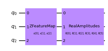
The first step to create a SamplerQNN is to define a parametrized feature map and ansatz. In this toy example, we will use 3 qubits and the QNNCircuit class to simplify the composition of a feature map and an ansatz circuit. The resulting circuit is then used in the SamplerQNN class.
[2]:
num_qubits = 3
# combine a custom feature map and ansatz into a single circuit
qc = QNNCircuit(
    feature_map=ZFeatureMap(feature_dimension=num_qubits, reps=1),
    ansatz=RealAmplitudes(num_qubits, reps=1),
)
qc.draw("mpl")
[2]:
The parametrized circuit can then be sent together with an optional interpret map (parity in this case) to the SamplerQNN constructor.
[3]:
# parity maps bitstrings to 0 or 1
def parity(x):
    return "{:b}".format(x).count("1") % 2


output_shape = 2  # corresponds to the number of classes, possible outcomes of the (parity) mapping.
[4]:
# construct QNN
qnn = SamplerQNN(
    circuit=qc,
    interpret=parity,
    output_shape=output_shape,
    sparse=False,
)
3.2 유효 차원 계산 설정#
EffectiveDimension 클래스를 사용해서 QNN의 유효 차원을 계산하려면, 데이터 세트에서 사용할 수 있는 전체 데이터 샘플 수를 비롯한 일련의 입력 샘플 및 가중치 세트가 필요하다. input_samples 과 weight_samples 는 클래스 생성자에서 설정하고, 데이터 샘플의 수는 유효 차원을 계산하는 호출에서 얻는다. 이로써 데이터 세트의 크기가 다를 경우 이러한 측정값이 어떻게 바뀌는지 테스트하고 비교할 수 있다.
사용자는 입력 샘플과 가중치 샘플의 수를 정의할 수 있으며 클래스는 정규(input_samples 의 경우) 또는 균일(weight_samples 의 경우) 분포에서 해당 배열을 무작위로 샘플링한다. 샘플의 갯수를 전달하는 대신 수동으로 샘플링된 배열을 전달할 수 있다.
[5]:
# we can set the total number of input samples and weight samples for random selection
num_input_samples = 10
num_weight_samples = 10

global_ed = EffectiveDimension(
    qnn=qnn, weight_samples=num_weight_samples, input_samples=num_input_samples
)
특정 세트의 입력 샘플과 가중치 샘플을 테스트하려는 경우 다음 스니펫과 같이 EffectiveDimension 클래스에 직접 전달할 수 있다.
[6]:
# we can also provide user-defined samples and parameters
input_samples = algorithm_globals.random.normal(0, 1, size=(10, qnn.num_inputs))
weight_samples = algorithm_globals.random.uniform(0, 1, size=(10, qnn.num_weights))

global_ed = EffectiveDimension(qnn=qnn, weight_samples=weight_samples, input_samples=input_samples)
유효 차원 알고리즘을 위해 데이터 세트 크기도 제공해야 한다. 이 예에서는 나중에 이 입력이 결과에 어떤 영향을 미치는지 확인하기 위해 크기 배열을 설정한다.
[7]:
# finally, we will define ranges to test different numbers of data, n
n = [5000, 8000, 10000, 40000, 60000, 100000, 150000, 200000, 500000, 1000000]
3.3 글로벌 유효 차원 계산#
Let’s now calculate the effective dimension of our network for the previously defined set of input samples, weights, and a dataset size of 5000.
[8]:
global_eff_dim_0 = global_ed.get_effective_dimension(dataset_size=n[0])
The effective dimension values will range between 0 and d, where d represents the dimension of the model, and it’s practically obtained from the number of weights of the QNN. By dividing the result by d, we can obtain the normalized effective dimension, which correlates directly with the capacity of the model.
[9]:
d = qnn.num_weights

print("Data size: {}, global effective dimension: {:.4f}".format(n[0], global_eff_dim_0))
print(
    "Number of weights: {}, normalized effective dimension: {:.4f}".format(d, global_eff_dim_0 / d)
)
Data size: 5000, global effective dimension: 4.6657
Number of weights: 6, normalized effective dimension: 0.7776
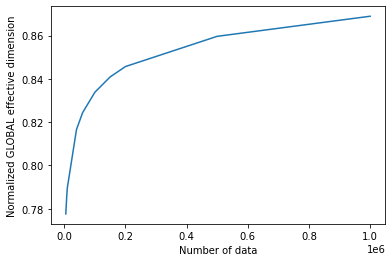
입력 크기가 n 인 경우 배열로 EffectiveDimension 클래스를 호출하면 데이터 세트 크기에 따라 유효 차원이 어떻게 변하는지 모니터링할 수 있다.
[10]:
global_eff_dim_1 = global_ed.get_effective_dimension(dataset_size=n)
[11]:
print("Effective dimension: {}".format(global_eff_dim_1))
print("Number of weights: {}".format(d))
Effective dimension: [4.66565096 4.7133723  4.73782922 4.89963559 4.94632272 5.00280009
 5.04530433 5.07408394 5.15786005 5.21349874]
Number of weights: 6
[12]:
# plot the normalized effective dimension for the model
plt.plot(n, np.array(global_eff_dim_1) / d)
plt.xlabel("Number of data")
plt.ylabel("Normalized GLOBAL effective dimension")
plt.show()
4. 로컬 유효 차원 예제#
앞에서 살펴본 것과 같이, 로컬 유효 차원 알고리즘은 하나의 가중치 집합만 사용하며 훈련이 신경망의 표현력에 미치는 영향을 모니터링하는 데 사용할 수 있다. LocalEffectiveDimension 클래스가 제약 조건을 적용함으로서 계산의 중요한 기능을 구현하는 동시에 계산의 나머지 부분은 EffectiveDimension 과 공유된다.
이 예제는 학습이 QNN 표현력에 미치는 영향을 분석하기 위해 LocalEffectiveDimension 클래스를 활용하는 방법을 보여준다.
4.1 데이터셋 및 QNN 정의#
We start by creating a 3D binary classification dataset using make_classification function from scikit-learn.
[13]:
num_inputs = 3
num_samples = 50

X, y = make_classification(
    n_samples=num_samples,
    n_features=num_inputs,
    n_informative=3,
    n_redundant=0,
    n_clusters_per_class=1,
    class_sep=2.0,
)
X = MinMaxScaler().fit_transform(X)
y = 2 * y - 1  # labels in {-1, 1}
The next step is to create a QNN, an instance of EstimatorQNN in our case in the same fashion we created an instance of SamplerQNN.
[14]:
estimator_qnn = EstimatorQNN(circuit=qc)
4.2 QNN 학습#
이제 QNN 학습을 시작해보자. 학습 단계는 다소 시간이 걸릴 수 있다. 학습 과정이 어떻게 진행되고 있는지 살펴보기 위해 분류기에 콜백을 전달할 수도 있다. 다른 예제에서와 같이 재현성을 위해 initial_point 를 고정한다.
[15]:
# callback function that draws a live plot when the .fit() method is called
def callback_graph(weights, obj_func_eval):
    clear_output(wait=True)
    objective_func_vals.append(obj_func_eval)
    plt.title("Objective function value against iteration")
    plt.xlabel("Iteration")
    plt.ylabel("Objective function value")
    plt.plot(range(len(objective_func_vals)), objective_func_vals)
    plt.show()
[16]:
# construct classifier
initial_point = algorithm_globals.random.random(estimator_qnn.num_weights)

estimator_classifier = NeuralNetworkClassifier(
    neural_network=estimator_qnn,
    optimizer=COBYLA(maxiter=80),
    initial_point=initial_point,
    callback=callback_graph,
)
[17]:
# create empty array for callback to store evaluations of the objective function (callback)
objective_func_vals = []
plt.rcParams["figure.figsize"] = (12, 6)

# fit classifier to data
estimator_classifier.fit(X, y)

# return to default figsize
plt.rcParams["figure.figsize"] = (6, 4)

만들어진 분류기는 아래와 같은 정확도로 클래스를 구별할 수 있다:
[18]:
# score classifier
estimator_classifier.score(X, y)
[18]:
0.96
4.3 학습된 QNN의 로컬 유효 차원 계산#
Now that we have trained our network, let’s evaluate the local effective dimension based on the trained weights. To do that we access the trained weights directly from the classifier.
[19]:
trained_weights = estimator_classifier.weights

# get Local Effective Dimension for set of trained weights
local_ed_trained = LocalEffectiveDimension(
    qnn=estimator_qnn, weight_samples=trained_weights, input_samples=X
)

local_eff_dim_trained = local_ed_trained.get_effective_dimension(dataset_size=n)

print(
    "normalized local effective dimensions for trained QNN: ",
    local_eff_dim_trained / estimator_qnn.num_weights,
)
normalized local effective dimensions for trained QNN:  [0.38001027 0.38667693 0.39017714 0.41507888 0.42307677 0.43341398
 0.44170977 0.44758111 0.46577231 0.4786767 ]
4.4 학습되지 않은 QNN의 로컬 유효 차원 계산#
가중치 샘플로 initial_point 를 사용하여 이 결과를 훈련되지 않은 네트워크의 유효 차원과 비교할 수 있다.
[20]:
# get Local Effective Dimension for set of untrained weights
local_ed_untrained = LocalEffectiveDimension(
    qnn=estimator_qnn, weight_samples=initial_point, input_samples=X
)

local_eff_dim_untrained = local_ed_untrained.get_effective_dimension(dataset_size=n)

print(
    "normalized local effective dimensions for untrained QNN: ",
    local_eff_dim_untrained / estimator_qnn.num_weights,
)
normalized local effective dimensions for untrained QNN:  [0.69803061 0.7130991  0.7203237  0.76321615 0.77452215 0.7877625
 0.79746712 0.8039319  0.82236146 0.83435907]
4.5 결과를 도식화 하고(Plot) 분석하기#
학습 전과 후의 유효 차원 값을 플롯하면 아래와 같은 결과를 볼 수 있다:
[21]:
# plot the normalized effective dimension for the model
plt.plot(n, np.array(local_eff_dim_trained) / estimator_qnn.num_weights, label="trained weights")
plt.plot(
    n, np.array(local_eff_dim_untrained) / estimator_qnn.num_weights, label="untrained weights"
)

plt.xlabel("Number of data")
plt.ylabel("Normalized LOCAL effective dimension")
plt.legend()
plt.show()
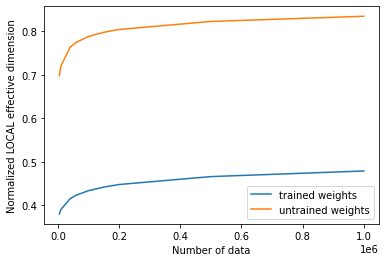
일반적으로 훈련 후에 로컬 유효 차원의 값이 감소할 것으로 예상할 수 있다. 이는 사용된 데이터에 적합할 만큼 표현력이 뛰어나면서도 과적합되어 새로운 데이터 샘플에 대해 성능이 나쁘지 않은 적절한 모델을 선택해야 하는 것과 같은, 머신 러닝의 중요한 목표와도 맥락을 같이 한다.
특정 옵티마이저는 매개변수를 학습하여 모델의 과적합을 조절하는데 도움을 주기도 하며 이 과정은 본질적으로 로컬 유효차원으로 측정할 수 있는 모덿의 표현력을 감소시킨다. 같은 논리로 무작위로 초기화된 매개 변수 세트는 훈련된 가중치의 최종 학습 세트보다 더 높은 유효차원을 가질 확률이 높으며, 이는 이 무작위 변수 세트를 지닌 모델이 데이터를 모두 맞추기 위해 불필요하게 ”더 많은 매개변수”를 사용하게 되기 때문이다. 학습이 종료 후(어느정도 조정이 이루어진) 학습된 모델은 더 적은 수의 매개변수를 사용해도 충분하기 때문에 더 많은 ”비활성 매개변수”와 더 낮은 유효 차원을 갖게 된다.
이것은 그저 보편적인 경우에 대한 통찰일 뿐이며 무작위로 선택된 가중치 세트가 특정 모델에 대해 훈련된 가중치보다 낮은 유효 차원을 제공하는 경우도 있음을 유념한다.
[22]:
import qiskit.tools.jupyter

%qiskit_version_table
%qiskit_copyright
Version Information
| Qiskit Software | Version |
|---|---|
qiskit-terra | 0.24.0 |
qiskit-aer | 0.12.0 |
qiskit-ignis | 0.6.0 |
qiskit-ibmq-provider | 0.20.2 |
qiskit | 0.43.0 |
qiskit-machine-learning | 0.7.0 |
| System information | |
| Python version | 3.8.8 |
| Python compiler | Clang 10.0.0 |
| Python build | default, Apr 13 2021 12:59:45 |
| OS | Darwin |
| CPUs | 8 |
| Memory (Gb) | 32.0 |
| Tue Jun 13 16:40:08 2023 CEST | |
This code is a part of Qiskit
© Copyright IBM 2017, 2023.
This code is licensed under the Apache License, Version 2.0. You may
obtain a copy of this license in the LICENSE.txt file in the root directory
of this source tree or at http://www.apache.org/licenses/LICENSE-2.0.
Any modifications or derivative works of this code must retain this
copyright notice, and modified files need to carry a notice indicating
that they have been altered from the originals.