Qiskit 기계 학습 v0.5 이전 안내#
이 지침서는 Qiskit Machine Learning v0.4 코드를 v0.5 로 이전시키는 과정을 안내한다.
소개#
Qiskit Machine Learning의 0.5 릴리즈 핵심은 알고리즘의 요소들에 대한 지원 뿐만 아니라 양자 커널(quantum kernels)과 양자 신경망(quantum neural networks)과 같은 기본 연산 블록들을 Qiskit의 요소로 이주하는 것이다.
내용:
요소의 개요
새 양자 커널
새 양자 신경망
기타 구식화된 것들
요소의 개요#
양자 컴퓨터가 고전 컴퓨터와 구분되는 핵심 기능은 출력으로 비고전적인 확률 분포를 생성하는 능력이다. 확률 분포를 직접적으로 다루는 연산은 샘플링을 하거나 값을 추정할 수 있어야 한다. 따라서, 이러한 샘플링 하거나 추론하는 연산자들은 양자 알고리즘 개발의 근본적인 빌딩 블록이 되어야 한다. 고로, 안내된 바 와 같이, 이 두 연산자들 Sampler와 Estimator가 기본 요소로 소개되었다:
Sampler 클래스는 양자 회로의 비트 문자열의 확률이나 준-확률을 계산한다. 기본 클래스는 qiskit.primitives.BaseSampler 이다.
Estimator 클래스는 양자 회로나 관측가능량의 기댓값을 추정한다. 기본 클래스는 qiskit.primitives.BaseEstimator 이다.
Qiskit Terra는 두 구현의 핵심 인터페이스를 제공한다:
이 참조 구현은 상태 벡터를 기반으로 한다. 이 구현은 백엔드나 시뮬레이터를 필요로 하며, quantum_info 패키지의 클래스들에 의존한다.
백엔드 기반 프리미티브는 프리미티브를 직접 지원하지 않는 공급자/백엔드를 지원하는 것이다. 이러한 구현에서는 프리미티브로 전달할 백엔드의 인스턴스가 필요하다.
Qiskit Terra 프리미티브에 관한 추가적인 정보는 문서 에서 찾을 수 있다.
다른 구현들도 언급할 가치가 있다.
Aer 프리미티브들은 반드시 Aer 시뮬레이터에 사용되어야 한다. 이것들은 Terra의 대응하는 인터페이스를 확장하며, Terra의 프리미티브들과 동일한 방식으로 사용될 수 있다. 추가적인 내용은 문서 를 참조하라.
IBM 장치들과 함께 사용될 런타임 프리미티브. 이는 실제 하드웨어상의 클라우드 컴퓨팅에 중점을 두고 있는 구현이다. 이곳 을 참조하라.
Along with the primitives Terra has some primitive-like algorithms that are highly useful in QML and used by the new 0.5 functions:
Algorithms to calculate the gradient of a quantum circuit. For each core primitive there’s a corresponding base interface that defines quantum circuit gradient. The documentation on gradients is here.
Algorithms that compute the fidelity or “closeness” of pairs of quantum states. Currently, only one implementation is available that requires a sampler primitive and is based on the compute-uncompute method. The documentation is here.
Both two new algorithms are very similar to the core primitives, they share the same method signatures, so they may be called as high level primitives despite they are not in the primitives package.
새 양자 커널#
The previous implementation consisted of a single class QuantumKernel that did everything:
Constructed circuits
Executed circuits and evaluated overlap between circuits
Provided training parameters
Kept track of the values assigned to the parameters.
The implementation became sophisticated and inflexible and adding support of the new primitives could be tricky. To address the issues, a new flexible and extendable design of quantum kernels was introduced. The goals of the new design are:
Migrate to the primitives and leverage the fidelity algorithm. Now users may plug in their own implementations of fidelity calculations.
Extract trainability feature to a dedicated class.
Introduce a base class that can be extended by other kernel implementations.
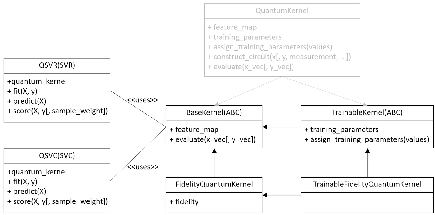
The new design of quantum kernel is shown on the next diagram.
The new kernels expose the same interface and the same parameters except
the quantum_instance parameter. This parameter does not have a
direct replacement and instead the fidelity parameter must be used.
The backend handling/selection, which was previously done using the
quantum_instance, is now taken care of via the Sampler primitive
given to the fidelity.
A new hierarchy shown on the diagram introduces:
A base and abstract class BaseKernel is introduced. All concrete implementation must inherit this class.
A fidelity based quantum kernel FidelityQuantumKernel is added. This is a direct replacement of the previous quantum kernel implementation. The difference is that the new class takes a fidelity instance to estimate overlaps and construct kernel matrix.
A new abstract class TrainableKernel is introduced to generalize ability to train quantum kernels.
A fidelity-based trainable quantum kernel TrainableFidelityQuantumKernel is introduced. This is a replacement of the previous quantum kernel if a trainable kernel is required. The trainer QuantumKernelTrainer now accepts both quantum kernel implementations, the new one and the previous one.
For convenience, the previous quantum kernel implementation, QuantumKernel, now extends both new abstract classes and thus it is compatible with the new introduced interfaces. This implementation is now pending deprecation, will be deprecated in a future release and subsequently removed after that. New, primitive-based quantum kernels should be used instead.
The existing algorithms such as QSVC, QSVR and other kernel-based algorithms are updated and work with both implementations.
For example a QSVM classifier can be trained as follows.
Create a dataset#
Fixing randomization.
from qiskit.utils import algorithm_globals

algorithm_globals.random_seed = 123456
Generate a simple dataset using scikit-learn.
from sklearn.datasets import make_blobs

features, labels = make_blobs(
    n_samples=20,
    centers=2,
    center_box=(-1, 1),
    cluster_std=0.1,
    random_state=algorithm_globals.random_seed,
)
Previous implementation of quantum kernel#
In the previous implementation we start from creating an instance of
QuantumInstance. This class defines where our quantum circuits are
executed. In this case we wrap a statevector simulator in the quantum
instance.
from qiskit import BasicAer
from qiskit.utils import QuantumInstance

sv_qi = QuantumInstance(
    BasicAer.get_backend("statevector_simulator"),
    seed_simulator=algorithm_globals.random_seed,
    seed_transpiler=algorithm_globals.random_seed,
)
Then create a quantum kernel.
from qiskit.circuit.library import ZZFeatureMap
from qiskit_machine_learning.kernels import QuantumKernel

feature_map = ZZFeatureMap(2)
previous_kernel = QuantumKernel(feature_map=feature_map, quantum_instance=sv_qi)
And finally we fit an SVM classifier.
from qiskit_machine_learning.algorithms import QSVC

qsvc = QSVC(quantum_kernel=previous_kernel)
qsvc.fit(features, labels)
qsvc.score(features, labels)
0.95
New implementation of quantum kernel#
In the new implementation we start from creating a Fidelity instance. Fidelity is optional and quantum kernel will create it automatically if none is passed. But here, we create it manually for illustrative purposes. To create a fidelity instance we pass a sampler. The sampler is the reference implementation and defines where our quantum circuits are executed. You may create a sampler instance from QiskitRuntimeService to leverage Qiskit runtime services.
from qiskit.algorithms.state_fidelities import ComputeUncompute
from qiskit.primitives import Sampler

fidelity = ComputeUncompute(sampler=Sampler())
Next, we create a new quantum kernel with the fidelity instance.
from qiskit_machine_learning.kernels import FidelityQuantumKernel

feature_map = ZZFeatureMap(2)
new_kernel = FidelityQuantumKernel(feature_map=feature_map, fidelity=fidelity)
Then we fit an SVM classifier the same way as before.
from qiskit_machine_learning.algorithms import QSVC

qsvc = QSVC(quantum_kernel=new_kernel)
qsvc.fit(features, labels)
qsvc.score(features, labels)
0.95
새 양자 신경망#
Changes in the quantum neural networks are not as dramatic as in quantum kernels. In addition, and as a replacement to the existing neural networks, two new networks are introduced. The new networks introduced are SamplerQNN and EstimatorQNN which are detailed below and are replacements for the pre-existing CircuitQNN, OpflowQNN and TwoLayerQNN which are now pending deprecated.
SamplerQNN#
A new Sampler Quantum Neural Network leverages the sampler primitive, sampler gradients and is a direct replacement of CircuitQNN.
The new
SamplerQNN
exposes a similar interface to the existing
CircuitQNN,
with a few differences. One is the quantum_instance parameter. This
parameter does not have a direct replacement, and instead the
sampler parameter must be used. The gradient parameter keeps the
same name as in the
CircuitQNN
implementation, but it no longer accepts Opflow gradient classes as
inputs; instead, this parameter expects an (optionally custom) primitive
gradient. The sampling option has been removed for the time being,
as this information is not currently exposed by the sampler, and might
correspond to future lower-level primitives.
The existing training algorithms such as VQC that were based on CircuitQNN, are updated to accept both implementations. The implementation of NeuralNetworkClassifier has not changed.
The existing CircuitQNN is now pending deprecation, will be deprecated in a future release and subsequently removed after that.
We’ll show how to train a variational quantum classifier using both networks. For this purposes we re-use the dataset generated for the quantum kernel. For both quantum neural networks we still have to construct a feature map, an ansatz and combine them into a single quantum circuit.
from qiskit import QuantumCircuit
from qiskit.circuit.library import RealAmplitudes

num_inputs = 2
feature_map = ZZFeatureMap(num_inputs)
ansatz = RealAmplitudes(num_inputs, reps=1)

circuit = QuantumCircuit(num_inputs)
circuit.compose(feature_map, inplace=True)
circuit.compose(ansatz, inplace=True)
We need an interpret function as well. We define our usual parity function that maps bitstrings either to \(0\) or \(1\).
def parity(x):
    return "{:b}".format(x).count("1") % 2
We fix the initial point to get the same results from both networks.
initial_point = algorithm_globals.random.random(ansatz.num_parameters)
Building a classifier using CircuitQNN#
We create a CircuitQNN instance and re-use the quantum instance
created for the quantum kernel.
from qiskit_machine_learning.neural_networks import CircuitQNN

circuit_qnn = CircuitQNN(
    circuit=circuit,
    input_params=feature_map.parameters,
    weight_params=ansatz.parameters,
    interpret=parity,
    output_shape=2,
    quantum_instance=sv_qi,
)
Construct a classifier out of the network, train it and score it. We are not aiming for good results, so the number of iterations is set to a small number to reduce overall execution time.
from qiskit.algorithms.optimizers import COBYLA
from qiskit_machine_learning.algorithms import NeuralNetworkClassifier

classifier = NeuralNetworkClassifier(
    neural_network=circuit_qnn,
    loss="cross_entropy",
    one_hot=True,
    optimizer=COBYLA(maxiter=40),
    initial_point=initial_point,
)
classifier.fit(features, labels)
classifier.score(features, labels)
0.6
Building a classifier using SamplerQNN#
Instead of QuantumInstance create an instance of the reference
Sampler.
from qiskit.primitives import Sampler

sampler = Sampler()
Now, we create a instance of SamplerQNN. The difference with
CircuitQNN is that we pass a sampler instead of a quantum instance.
from qiskit_machine_learning.neural_networks import SamplerQNN

sampler_qnn = SamplerQNN(
    circuit=circuit,
    input_params=feature_map.parameters,
    weight_params=ansatz.parameters,
    interpret=parity,
    output_shape=2,
    sampler=sampler,
)
Construct a classifier and fit it as usual. As neural_network we
pass a created SamplerQNN and this is the only difference.
classifier = NeuralNetworkClassifier(
    neural_network=sampler_qnn,
    loss="cross_entropy",
    one_hot=True,
    optimizer=COBYLA(maxiter=40),
    initial_point=initial_point,
)
classifier.fit(features, labels)
classifier.score(features, labels)
0.6
Instead of constructing a quantum neural network manually, you may train
VQC. It takes either a quantum instance or a sampler, depending on
what is passed it automatically constructs either CircuitQNN or
SamplerQNN respectively.
EstimatorQNN#
A new Estimator quantum neural network leverages the estimator primitive, estimator gradients and is a direct replacement of OpflowQNN.
The new
EstimatorQNN
exposes a similar interface to the existing
OpflowQNN,
with a few differences. One is the quantum_instance parameter. This
parameter does not have a direct replacement, and instead the
estimator parameter must be used. The gradient parameter keeps
the same name as in the
OpflowQNN
implementation, but it no longer accepts Opflow gradient classes as
inputs; instead, this parameter expects an (optionally custom) primitive
gradient.
The existing training algorithms such as VQR that were based on the TwoLayerQNN, are updated to accept both implementations. The implementation of NeuralNetworkRegressor has not changed.
The existing OpflowQNN is now pending deprecation, will be deprecated in a future release and subsequently removed after that.
We’ll show how to train a variational quantum regressor using both networks. We start from generating a simple regression dataset.
import numpy as np

num_samples = 20
eps = 0.2
lb, ub = -np.pi, np.pi
features = (ub - lb) * np.random.rand(num_samples, 1) + lb
labels = np.sin(features[:, 0]) + eps * (2 * np.random.rand(num_samples) - 1)
We still have to construct a feature map, an ansatz and combine them into a single quantum circuit for both quantum neural networks.
from qiskit.circuit import Parameter

num_inputs = 1
feature_map = QuantumCircuit(1)
feature_map.ry(Parameter("input"), 0)

ansatz = QuantumCircuit(1)
ansatz.ry(Parameter("weight"), 0)

circuit = QuantumCircuit(num_inputs)
circuit.compose(feature_map, inplace=True)
circuit.compose(ansatz, inplace=True)
We fix the initial point to get the same results from both networks.
initial_point = algorithm_globals.random.random(ansatz.num_parameters)
Building a regressor using OpflowQNN#
We create an OpflowQNN instance and re-use the quantum instance
created for the quantum kernel.
from qiskit.opflow import PauliSumOp, StateFn
from qiskit_machine_learning.neural_networks import OpflowQNN

observable = PauliSumOp.from_list([("Z", 1)])
operator = StateFn(observable, is_measurement=True) @ StateFn(circuit)

opflow_qnn = OpflowQNN(
    operator=operator,
    input_params=feature_map.parameters,
    weight_params=ansatz.parameters,
    quantum_instance=sv_qi,
)
Construct a regressor out of the network, train it and score it. In this case we use a gradient based optimizer, thus the network makes use of the gradient framework and due to nature of the dataset converges very quickly.
from qiskit.algorithms.optimizers import L_BFGS_B
from qiskit_machine_learning.algorithms import NeuralNetworkRegressor

regressor = NeuralNetworkRegressor(
    neural_network=opflow_qnn,
    optimizer=L_BFGS_B(maxiter=5),
    initial_point=initial_point,
)
regressor.fit(features, labels)
regressor.score(features, labels)
0.9681198723451012
Building a regressor using EstimatorQNN#
Create an instance of the reference Estimator. You may create an estimator instance from QiskitRuntimeService to leverage Qiskit runtime services.
from qiskit.primitives import Estimator

estimator = Estimator()
Now, we create a instance of EstimatorQNN. The network creates an
observable as \(Z^{\otimes n}\), where \(n\) is the number of
qubit, if it is not specified.
from qiskit_machine_learning.neural_networks import EstimatorQNN

estimator_qnn = EstimatorQNN(
    circuit=circuit,
    input_params=feature_map.parameters,
    weight_params=ansatz.parameters,
    estimator=estimator,
)
Construct a variational quantum regressor and fit it. In this case we use a gradient based optimizer, thus the network makes use of the default estimator gradient that is created automatically.
from qiskit.algorithms.optimizers import L_BFGS_B
from qiskit_machine_learning.algorithms import VQR

regressor = NeuralNetworkRegressor(
    neural_network=estimator_qnn,
    optimizer=L_BFGS_B(maxiter=5),
    initial_point=initial_point,
)
regressor.fit(features, labels)
regressor.score(features, labels)
0.9681198723451012
Instead of constructing a quantum neural network manually, you may train
VQR. It takes either a quantum instance or an estimator, depending
on what is passed it automatically constructs either TwoLayerQNN or
EstimatorQNN respectively.
기타 구식화된 것들#
A few other components, not mentioned explicitly above, are also deprecated or pending deprecation:
TwoLayerQNN is pending deprecation. Users should use EstimatorQNN instead.
The Distribution Learners package is deprecated fully. This package contains such classes as DiscriminativeNetwork, GenerativeNetwork, NumPyDiscriminator, PyTorchDiscriminator, QuantumGenerator, QGAN. Instead, please refer to the new QGAN tutorial. This tutorial introduces step-by-step how to build a PyTorch-based QGAN using quantum neural networks.
The Runtime package is deprecated. This package contains a client to Qiskit Programs that embed Qiskit Runtime in the algorithmic interfaces and facilitate usage of algorithms and scripts in the cloud. You should use QiskitRuntimeService to leverage primitives and runtimes.
import qiskit.tools.jupyter

%qiskit_version_table
%qiskit_copyright
Version Information
| Qiskit Software | Version |
|---|---|
qiskit-terra | 0.25.0 |
qiskit-aer | 0.13.0 |
qiskit-machine-learning | 0.7.0 |
| System information | |
| Python version | 3.8.13 |
| Python compiler | Clang 12.0.0 |
| Python build | default, Oct 19 2022 17:54:22 |
| OS | Darwin |
| CPUs | 10 |
| Memory (Gb) | 64.0 |
| Thu Sep 14 13:57:31 2023 IST | |
This code is a part of Qiskit
© Copyright IBM 2017, 2023.
This code is licensed under the Apache License, Version 2.0. You may
obtain a copy of this license in the LICENSE.txt file in the root directory
of this source tree or at http://www.apache.org/licenses/LICENSE-2.0.
Any modifications or derivative works of this code must retain this
copyright notice, and modified files need to carry a notice indicating
that they have been altered from the originals.