注釈

このページは docs/tutorials/04_torch_qgan.ipynb から生成されました。

PyTorchによるqGANの実装

概要

このチュートリアルでは、PyTorchベースの量子敵対的生成ネットワークのアルゴリズムを構築する方法をステップバイステップで紹介します。

このチュートリアルの構造は以下のとおりです。

1. はじめに

2. データと表現

3. ニューラルネットワークの定義

4. トレーニング・ループのセットアップ

5. モデルのトレーニング

6. 結果: 累積密度関数

7. 結論

1. はじめに

qGAN [1]は、生成モデリングを行うために使用されるハイブリッド量子古典アルゴリズムです。このアルゴリズムでは、量子生成器 \(G_{\theta}\) つまり ansatz (パラメーター化された量子回路) と古典識別器 \(D_{\phi}\) (ニューラルネットワーク) の相互作用により、トレーニングデータから基礎となる確率分布の学習を行います。

生成器と識別器は交互に最適化され、生成器は識別器が学習データ値として分類する確率（実際の学習分布から抽出した確率）の生成を目指し、識別器は元の分布と生成器からの確率を区別する（つまり、実際の分布と生成した分布を区別する）ことを目指します。最終的な目標は、量子生成器が目的とする確率分布の表現を学習することです。この学習により、量子生成器は、ターゲット分布の近似モデルである量子状態をロードするために使用することができます。

**参考文献: **

[1] Zoufal et al., Quantum Generative Adversarial Networks for learning and loading random distributions

1.1 ランダム分布をロードするためのqGAN

\(k\) 次元のデータサンプルが与えられた場合、量子敵対的生成ネットワーク (qGAN) を使用してランダム分布を学習し、それを量子状態に直接ロードします。

\[\big| g_{\theta}\rangle = \sum_{j=0}^{2^n-1} \sqrt{p_{\theta}^{j}}\big| j \rangle\]

ここで \(p_{\theta}^{j}\) は、基底状態 \(\big| j\rangle\) の発生確率を表します。

qGAN学習の目的は、状態 \(\big| g_{\theta}\rangle\) を生成することです。ここで、 \(p_{\theta}^{j}\) は、 \(j\in \left\{0, \ldots, {2^n-1} \right\}\) の場合、 学習データ \(X=\left\{x^0, \ldots, x^{k-1} \right\}\) の基礎となる分布に近い確率分布を表します。

詳細については、 Quantum Generative Adversarial Networks for Learning and Loading Random Distributions Zoufal, Lucchi, Woerner [2019] を参照してください。

学習済みの qGAN の実用例として、金融デリバティブの価格設定については、チュートリアルの qGANs によるオプション価格推定 を参照してください。

データと表現

まず、学習データ \(X\) をロードする必要があります。

このチュートリアルでは、訓練データは2次元多変量正規分布によって与えられます。

生成器の目標は、そのような分布を表す方法を学習することであり、トレーニングされた生成器は \(n\)-qubit 量子状態に対応する必要があります \begin{equation} |g_{\text{trained }}\rangle=\sum\limits_{j=0}^{k-1}\sqrt{p_{j}}|x_{j}\rangle, \end{equation} ここで、基底状態 \(|x_{j}\rangle\) はトレーニング データ セット内のデータ項目を表します \(X={x_0, \ldots, x_{k-1}}\) with :math:` kleq 2^n` と \(p_j\) は \(|x_{j}\rangle\) のサンプリング確率を指します。

この表現を容易にするために、多変量正規分布からのサンプルを離散的な値にマッピングする必要があります。表現できる値の数はマッピングに使用する量子ビットの数に依存します。したがって、データの分解能は量子ビットの数によって定義されます。math:3 個の量子ビットを使って 1 つの特徴を表現すると、 \(2^3 = 8\) 個の離散値を持つことになります。

まず、このチュートリアルでは、結果の再現性を得るために乱数ジェネレータのシードを固定します。

import torch
from qiskit.utils import algorithm_globals

algorithm_globals.random_seed = 123456
_ = torch.manual_seed(123456)  # suppress output

次元の数、離散数を固定し、 \(2^3 = 8\) として必要な量子ビット数を計算します。

import numpy as np

num_dim = 2
num_discrete_values = 8
num_qubits = num_dim * int(np.log2(num_discrete_values))

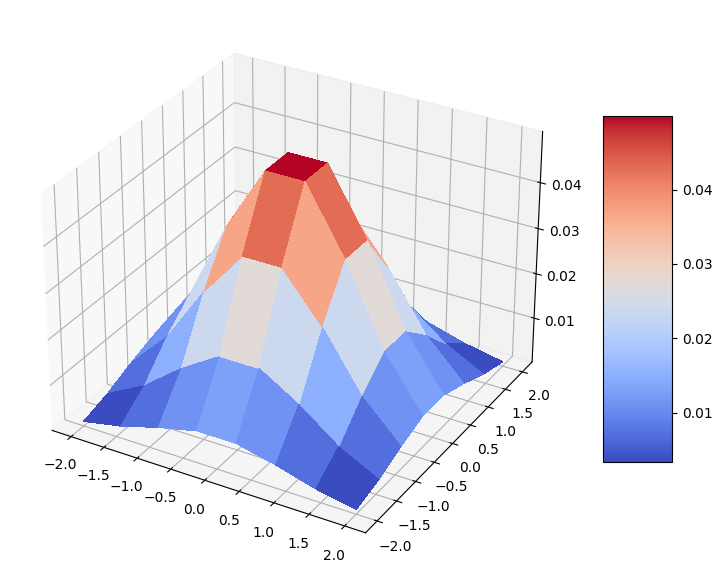
次に、連続2次元正規分布から離散分布を準備します。特徴ごとに \(8\) 個の値で離散化された、 \((-2, 2)^2\) 格子上の連続確率密度関数 (probability density function, PDF) を評価します。したがって、PDFの値は \(64\) となります。これは離散分布になるので、得られた確率を正規化します。

from scipy.stats import multivariate_normal

coords = np.linspace(-2, 2, num_discrete_values)
rv = multivariate_normal(mean=[0.0, 0.0], cov=[[1, 0], [0, 1]], seed=algorithm_globals.random_seed)
grid_elements = np.transpose([np.tile(coords, len(coords)), np.repeat(coords, len(coords))])
prob_data = rv.pdf(grid_elements)
prob_data = prob_data / np.sum(prob_data)

我々の分布を可視化しましょう。離散格子上の素敵なベル型の二変量正規分布です。

import matplotlib.pyplot as plt
from matplotlib import cm

mesh_x, mesh_y = np.meshgrid(coords, coords)
grid_shape = (num_discrete_values, num_discrete_values)

fig, ax = plt.subplots(figsize=(9, 9), subplot_kw={"projection": "3d"})
prob_grid = np.reshape(prob_data, grid_shape)
surf = ax.plot_surface(mesh_x, mesh_y, prob_grid, cmap=cm.coolwarm, linewidth=0, antialiased=False)
fig.colorbar(surf, shrink=0.5, aspect=5)
plt.show()

3. ニューラルネットワークの定義

このセクションでは、上記の2つのニューラルネットワークを定義します。

• 量子ニューラルネットワークとしての量子生成器。

• PyTorchベースのニューラルネットワークとしての古典的な識別器。

3.1. 量子ニューラルネットワークansatzの定義

ここで、量子生成器に用いるパラメータ化量子回路 \(G\left(\boldsymbol{\theta}\right)\) を \(\boldsymbol{\theta} = {\theta_1, ..., \theta_k}\) で定義します。 これは、量子生成器で使用されます。

量子生成器を実装するために、ハードウェア的に効率的な、\(6\) 回繰り返しのansatzを選択します。このansatzは \(R_Y\), \(R_Z\) 回転と \(CX\) ゲートを実装し、入力状態として一様分布を受け取ります。特に \(k>1\) の場合、生成器のパラメーターは注意深く選択する必要があります。例えば、回路の深さは \(1\) 以上であるべきです。これは、回路の深さが大きいほど、より複雑な構造を表現できるからです。ここでは、分布を適切にとらえて表現できるように、多くのパラメーターを持つかなり深い回路を構築します。

from qiskit import QuantumCircuit
from qiskit.circuit.library import EfficientSU2

qc = QuantumCircuit(num_qubits)
qc.h(qc.qubits)

ansatz = EfficientSU2(num_qubits, reps=6)
qc.compose(ansatz, inplace=True)

回路を描いて、どのように見えるか確認してみましょう。プロット上に \(6\) 回現れるパターンに気づくかもしれません。

qc.decompose().draw("mpl")

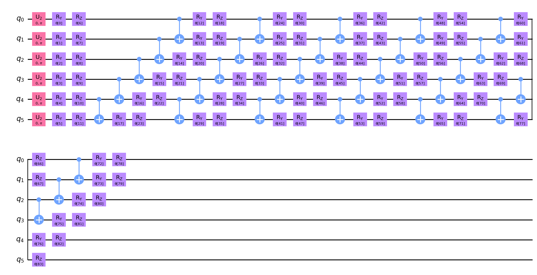
トレーニング可能なパラメーターの数を表示しましょう。

qc.num_parameters

84

3.2. 量子生成器の定義

Ansatz 用のサンプラーを作成することで、生成器の定義を開始します。 リファレンス実装は状態ベクトルベースの実装であり、回路実行の結果として正確な確率を返します。 結果にノイズを追加するために shots パラメーターを追加します。 この場合、実装は、測定された準確率から構築された多変量正規分布からの確率をサンプルします。 そして、いつものように再現性の目的のためにシードを固定します。

from qiskit.primitives import Sampler

shots = 10000
sampler = Sampler(options={"shots": shots, "seed": algorithm_globals.random_seed})

次に、パラメーター化された量子回路から量子生成器を作成する関数を定義します。この関数の中には、基礎となるサンプラーによって評価された準確率分布を返すニューラルネットワークを作成します。再現性のために initial_weights を固定します。作成された量子ニューラルネットワークを TorchConnector でラップし、PyTorch ベースのトレーニングを利用できるようにします。

from qiskit_machine_learning.connectors import TorchConnector
from qiskit_machine_learning.neural_networks import SamplerQNN


def create_generator() -> TorchConnector:
    qnn = SamplerQNN(
        circuit=qc,
        sampler=sampler,
        input_params=[],
        weight_params=qc.parameters,
        sparse=False,
    )

    initial_weights = algorithm_globals.random.random(qc.num_parameters)
    return TorchConnector(qnn, initial_weights)

3.3. 古典識別子の定義

次に、古典的な識別器を表すPyTorchベースの古典的ニューラルネットワークを定義します。基礎となる勾配はPyTorchで自動的に計算することができます。

from torch import nn


class Discriminator(nn.Module):
    def __init__(self, input_size):
        super(Discriminator, self).__init__()

        self.linear_input = nn.Linear(input_size, 20)
        self.leaky_relu = nn.LeakyReLU(0.2)
        self.linear20 = nn.Linear(20, 1)
        self.sigmoid = nn.Sigmoid()

    def forward(self, input: torch.Tensor) -> torch.Tensor:
        x = self.linear_input(input)
        x = self.leaky_relu(x)
        x = self.linear20(x)
        x = self.sigmoid(x)
        return x

3.4. 生成器と識別器を作成する

次に、私たちは、生成器と識別器を作成します。

generator = create_generator()
discriminator = Discriminator(num_dim)

4. トレーニング・ループのセットアップ

このセクションでは以下をセットアップします。

• 生成器と識別器の損失関数。

• 両方に対するオプティマイザー。

• トレーニングプロセスを視覚化するユーティリティプロット関数。

4.1. 損失関数の定義

損失関数として2値クロスエントロピーを用い、生成器と識別器を学習させたいと思います。

\[L\left(\boldsymbol{\theta}\right)=\sum_jp_j\left(\boldsymbol{\theta}\right)\left[y_j\log(x_j) + (1-y_j)\log(1-x_j)\right],\]

ここで、 \(x_j\) はデータサンプル、 \(y_j\) はそれに対応するラベルを表します。

PyTorchの binary_cross_entropy は重みに関して微分できないため、勾配を評価できるように手動で損失関数を実装しています。

def adversarial_loss(input, target, w):
    bce_loss = target * torch.log(input) + (1 - target) * torch.log(1 - input)
    weighted_loss = w * bce_loss
    total_loss = -torch.sum(weighted_loss)
    return total_loss

4.2. オプティマイザーの定義

生成器と識別器を学習させるためには、最適化スキームを定義する必要があります。以下では、Adamと呼ばれる運動量ベースの最適化手法を採用します。詳しくは Kingma et al., Adam: A method for stochastic optimization を参照してください。

from torch.optim import Adam

lr = 0.01  # learning rate
b1 = 0.7  # first momentum parameter
b2 = 0.999  # second momentum parameter

generator_optimizer = Adam(generator.parameters(), lr=lr, betas=(b1, b2), weight_decay=0.005)
discriminator_optimizer = Adam(
    discriminator.parameters(), lr=lr, betas=(b1, b2), weight_decay=0.005
)

4.3. トレーニングプロセスの可視化

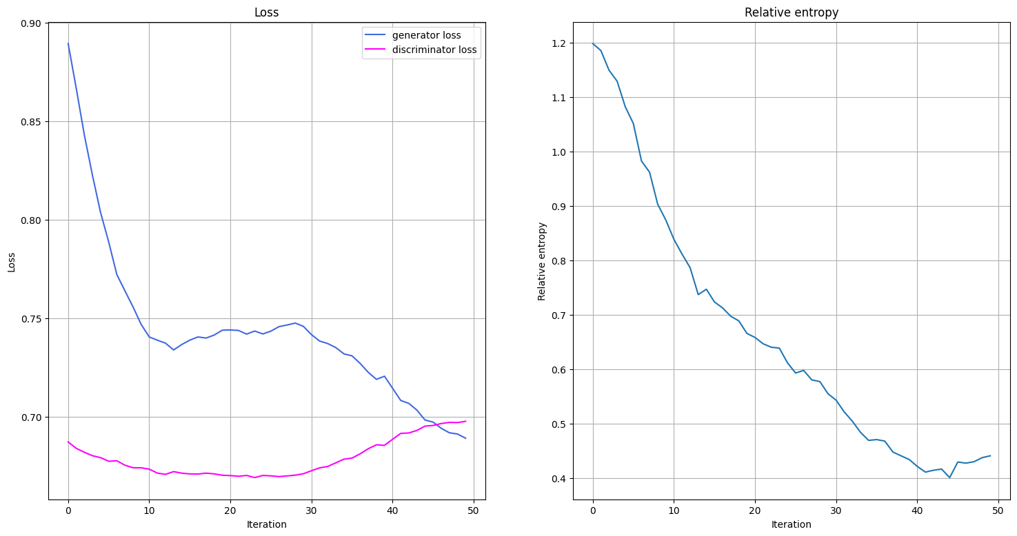
トレーニング中の生成器と識別器の損失関数の推移と、トレーニング後の分布とターゲット分布の相対エントロピーの推移をプロットすることで、トレーニング中に何が起こっているかを可視化します。損失関数と相対エントロピーのプロットを行う関数を定義します。この関数は、1エポックのトレーニングが終了した時点で呼び出されます。

学習過程の可視化は、2つのエポックに渡って学習データが収集された時点から開始されます。

from IPython.display import clear_output


def plot_training_progress():
    # we don't plot if we don't have enough data
    if len(generator_loss_values) < 2:
        return

    clear_output(wait=True)
    fig, (ax1, ax2) = plt.subplots(1, 2, figsize=(18, 9))

    # Generator Loss
    ax1.set_title("Loss")
    ax1.plot(generator_loss_values, label="generator loss", color="royalblue")
    ax1.plot(discriminator_loss_values, label="discriminator loss", color="magenta")
    ax1.legend(loc="best")
    ax1.set_xlabel("Iteration")
    ax1.set_ylabel("Loss")
    ax1.grid()

    # Relative Entropy
    ax2.set_title("Relative entropy")
    ax2.plot(entropy_values)
    ax2.set_xlabel("Iteration")
    ax2.set_ylabel("Relative entropy")
    ax2.grid()

    plt.show()

5. モデルのトレーニング

トレーニング・ループでは、損失関数だけでなく、相対エントロピーも監視します。相対エントロピーは分布の距離指標を表します。 したがって、これを使用して、トレーニングされた分布がターゲット分布からどれだけ近い/遠くにあるかをベンチマークすることができます。

これで、モデルを学習させる準備が整いました。モデルのトレーニングには時間がかかるかもしれませんので、気長にお待ちください。

import time
from scipy.stats import multivariate_normal, entropy

n_epochs = 50

num_qnn_outputs = num_discrete_values**num_dim

generator_loss_values = []
discriminator_loss_values = []
entropy_values = []

start = time.time()
for epoch in range(n_epochs):

    valid = torch.ones(num_qnn_outputs, 1, dtype=torch.float)
    fake = torch.zeros(num_qnn_outputs, 1, dtype=torch.float)

    # Configure input
    real_dist = torch.tensor(prob_data, dtype=torch.float).reshape(-1, 1)

    # Configure samples
    samples = torch.tensor(grid_elements, dtype=torch.float)
    disc_value = discriminator(samples)

    # Generate data
    gen_dist = generator(torch.tensor([])).reshape(-1, 1)

    # Train generator
    generator_optimizer.zero_grad()
    generator_loss = adversarial_loss(disc_value, valid, gen_dist)

    # store for plotting
    generator_loss_values.append(generator_loss.detach().item())

    generator_loss.backward(retain_graph=True)
    generator_optimizer.step()

    # Train Discriminator
    discriminator_optimizer.zero_grad()

    real_loss = adversarial_loss(disc_value, valid, real_dist)
    fake_loss = adversarial_loss(disc_value, fake, gen_dist.detach())
    discriminator_loss = (real_loss + fake_loss) / 2

    # Store for plotting
    discriminator_loss_values.append(discriminator_loss.detach().item())

    discriminator_loss.backward()
    discriminator_optimizer.step()

    entropy_value = entropy(gen_dist.detach().squeeze().numpy(), prob_data)
    entropy_values.append(entropy_value)

    plot_training_progress()

elapsed = time.time() - start
print(f"Fit in {elapsed:0.2f} sec")

Fit in 70.86 sec

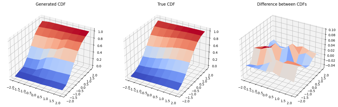
6. 結果: 累積密度関数

このセクションでは、トレーニングした分布の累積分布関数 (cumulative distribution function, CDF) とターゲット分布の CDF を比較します。

まず、モデルをもうトレーニングしないので、PyTorch の autograd をオフにして新しい確率分布を生成します。

with torch.no_grad():
    generated_probabilities = generator().numpy()

そして、生成された分布と元の分布の累積分布関数、そしてそれらの差をプロットします。注意してください。3 番目のプロットのスケールは 1 番目と 2 番目のプロットと 同じではありません 。

fig = plt.figure(figsize=(18, 9))

# Generated CDF
gen_prob_grid = np.reshape(np.cumsum(generated_probabilities), grid_shape)

ax1 = fig.add_subplot(1, 3, 1, projection="3d")
ax1.set_title("Generated CDF")
ax1.plot_surface(mesh_x, mesh_y, gen_prob_grid, linewidth=0, antialiased=False, cmap=cm.coolwarm)
ax1.set_zlim(-0.05, 1.05)

# Real CDF
real_prob_grid = np.reshape(np.cumsum(prob_data), grid_shape)

ax2 = fig.add_subplot(1, 3, 2, projection="3d")
ax2.set_title("True CDF")
ax2.plot_surface(mesh_x, mesh_y, real_prob_grid, linewidth=0, antialiased=False, cmap=cm.coolwarm)
ax2.set_zlim(-0.05, 1.05)

# Difference
ax3 = fig.add_subplot(1, 3, 3, projection="3d")
ax3.set_title("Difference between CDFs")
ax3.plot_surface(
    mesh_x, mesh_y, real_prob_grid - gen_prob_grid, linewidth=2, antialiased=False, cmap=cm.coolwarm
)
ax3.set_zlim(-0.05, 0.1)
plt.show()

7. 結論

量子敵対的生成ネットワークは、生成器と識別器の相互作用により、与えられたデータサンプルの下にある確率分布の近似表現を量子チャンネルにマッピングするものです。このチュートリアルでは、生成器を量子チャネル、すなわち変分量子回路、識別器を古典的なニューラルネットワークとして、PyTorch ベースの qGAN の実装を紹介し、一般的な確率分布の効率的な学習と量子状態へロードする応用について議論しました。この近似的なローディングには \(\mathscr{O}\left(poly\left(n\right)\right)\) 個のゲートが必要であり、潜在的に有利な量子アルゴリズムを利用できます。

import qiskit.tools.jupyter

%qiskit_version_table
%qiskit_copyright

Version Information

Qiskit Software	Version
qiskit-terra	0.23.1
qiskit-aer	0.12.0
qiskit-machine-learning	0.6.0
System information
Python version	3.8.13
Python compiler	Clang 12.0.0
Python build	default, Oct 19 2022 17:54:22
OS	Darwin
CPUs	10
Memory (Gb)	64.0
Mon Feb 20 17:09:10 2023 GMT

This code is a part of Qiskit

© Copyright IBM 2017, 2023.

This code is licensed under the Apache License, Version 2.0. You may
obtain a copy of this license in the LICENSE.txt file in the root directory
of this source tree or at http://www.apache.org/licenses/LICENSE-2.0.

Any modifications or derivative works of this code must retain this
copyright notice, and modified files need to carry a notice indicating
that they have been altered from the originals.