Note
Cette page a été générée à partir de docs/tutorials/02_neural_network_classifier_and_regressor.ipynb.
Classification et régression de réseau de neurones#
Dans ce tutoriel, nous montrons comment utiliser NeuralNetworkClassifier et NeuralNetworkRegressor. Les deux prennent comme entrée (Quantique) NeuralNetwork et l’exploitent dans un contexte spécifique. Dans les deux cas, nous proposons également pour plus de commodité, une variante préconfigurée : Le Classificateur Variationnel Quantique (VQC) et le Régresseur Variationnel Quantique (VQR). Le didacticiel est structuré comme suit :
Classification <#Classification> __
Classification avec
EstimatorQNNClassification avec un
SamplerQNNClassifieur Variationnel Quantique (VQC)
Régression <#Regression> __
Classification avec
EstimatorQNNRégresseur Variationnel Quantique (
VQR)
[1]:
import matplotlib.pyplot as plt
import numpy as np
from IPython.display import clear_output
from qiskit import QuantumCircuit
from qiskit.circuit import Parameter
from qiskit.circuit.library import RealAmplitudes, ZZFeatureMap
from qiskit_algorithms.optimizers import COBYLA, L_BFGS_B
from qiskit_algorithms.utils import algorithm_globals

from qiskit_machine_learning.algorithms.classifiers import NeuralNetworkClassifier, VQC
from qiskit_machine_learning.algorithms.regressors import NeuralNetworkRegressor, VQR
from qiskit_machine_learning.neural_networks import SamplerQNN, EstimatorQNN
from qiskit_machine_learning.circuit.library import QNNCircuit

algorithm_globals.random_seed = 42
Classification#
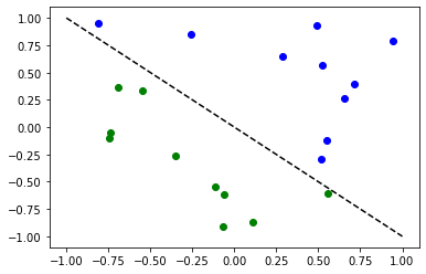
Nous préparons un ensemble de données de classification simple pour illustrer les algorithmes suivants.
[2]:
num_inputs = 2
num_samples = 20
X = 2 * algorithm_globals.random.random([num_samples, num_inputs]) - 1
y01 = 1 * (np.sum(X, axis=1) >= 0)  # in { 0,  1}
y = 2 * y01 - 1  # in {-1, +1}
y_one_hot = np.zeros((num_samples, 2))
for i in range(num_samples):
    y_one_hot[i, y01[i]] = 1

for x, y_target in zip(X, y):
    if y_target == 1:
        plt.plot(x[0], x[1], "bo")
    else:
        plt.plot(x[0], x[1], "go")
plt.plot([-1, 1], [1, -1], "--", color="black")
plt.show()
Classification avec EstimatorQNN#
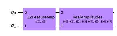
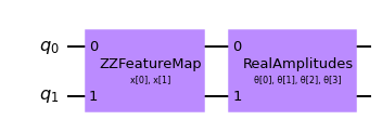
First we show how an EstimatorQNN can be used for classification within a NeuralNetworkClassifier. In this context, the EstimatorQNN is expected to return one-dimensional output in \([-1, +1]\). This only works for binary classification and we assign the two classes to \(\{-1, +1\}\). To simplify the composition of parameterized quantum circuit from a feature map and an ansatz we can use the QNNCircuit class.
[3]:
# construct QNN with the QNNCircuit's default ZZFeatureMap feature map and RealAmplitudes ansatz.
qc = QNNCircuit(num_qubits=2)
qc.draw(output="mpl")
[3]:
Création d’un réseau de neurones quantique
[4]:
estimator_qnn = EstimatorQNN(circuit=qc)
[5]:
# QNN maps inputs to [-1, +1]
estimator_qnn.forward(X[0, :], algorithm_globals.random.random(estimator_qnn.num_weights))
[5]:
array([[0.23521988]])
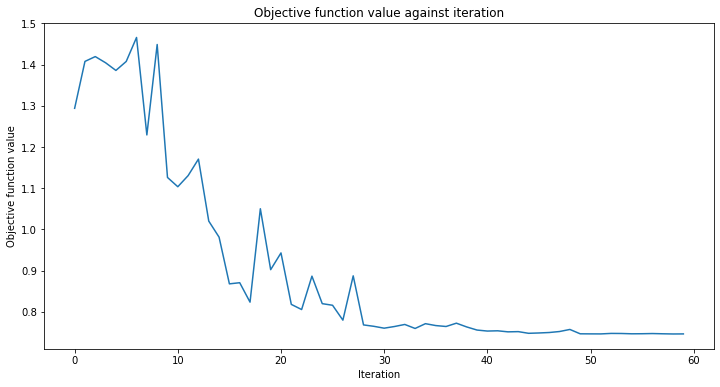
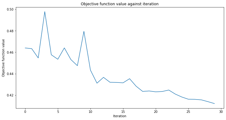
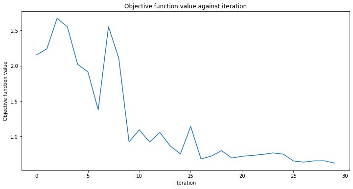
Nous allons ajouter une fonction de rappel appelée callback_graph. Elle sera appelée pour chaque itération de l’optimiseur et recevra deux paramètres : les poids actuels et la valeur de la fonction objectif à ces pondérations. Pour notre fonction, nous ajoutons la valeur de la fonction objectif à un tableau pour que nous puissions tracer la valeur de l’itération par rapport à la fonction objectif et mettre à jour le graphe avec chaque itération. Cependant, vous pouvez faire ce que vous voulez avec une fonction de rappel tant qu’elle obtient les deux paramètres mentionnés.
[6]:
# callback function that draws a live plot when the .fit() method is called
def callback_graph(weights, obj_func_eval):
    clear_output(wait=True)
    objective_func_vals.append(obj_func_eval)
    plt.title("Objective function value against iteration")
    plt.xlabel("Iteration")
    plt.ylabel("Objective function value")
    plt.plot(range(len(objective_func_vals)), objective_func_vals)
    plt.show()
[7]:
# construct neural network classifier
estimator_classifier = NeuralNetworkClassifier(
    estimator_qnn, optimizer=COBYLA(maxiter=60), callback=callback_graph
)
[8]:
# create empty array for callback to store evaluations of the objective function
objective_func_vals = []
plt.rcParams["figure.figsize"] = (12, 6)

# fit classifier to data
estimator_classifier.fit(X, y)

# return to default figsize
plt.rcParams["figure.figsize"] = (6, 4)

# score classifier
estimator_classifier.score(X, y)
[8]:
0.8
[9]:
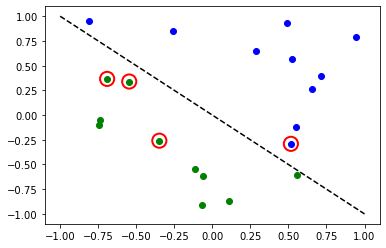
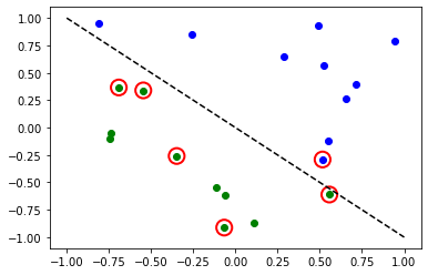
# evaluate data points
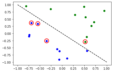
y_predict = estimator_classifier.predict(X)
# plot results
# red == wrongly classified
for x, y_target, y_p in zip(X, y, y_predict):
if y_target == 1:
plt.plot(x[0], x[1], "bo")
else:
plt.plot(x[0], x[1], "go")
if y_target != y_p:
plt.scatter(x[0], x[1], s=200, facecolors="none", edgecolors="r", linewidths=2)
plt.plot([-1, 1], [1, -1], "--", color="black")
plt.show()
Maintenant, quand le modèle est entraîné, nous pouvons explorer les poids du réseau neuronal. Veuillez noter que le nombre de poids est défini par ansatz.
[10]:
estimator_classifier.weights
[10]:
array([ 7.99142399e-01, -1.02869770e+00, -1.32131512e-04, -3.47046684e-01,
        1.13636802e+00,  6.56831727e-01,  2.17902158e+00, -1.08678332e+00])
Classification avec un SamplerQNN#
Next we show how a SamplerQNN can be used for classification within a NeuralNetworkClassifier. In this context, the SamplerQNN is expected to return \(d\)-dimensional probability vector as output, where \(d\) denotes the number of classes. The underlying Sampler primitive returns quasi-distributions of bit strings and we just need to define a mapping from the measured bitstrings to the different classes. For binary classification we use the parity mapping. Again we can
use the QNNCircuit class to set up a parameterized quantum circuit from a feature map and ansatz of our choice.
[11]:
# construct a quantum circuit from the default ZZFeatureMap feature map and a customized RealAmplitudes ansatz
qc = QNNCircuit(ansatz=RealAmplitudes(num_inputs, reps=1))
qc.draw(output="mpl")
[11]:
[12]:
# parity maps bitstrings to 0 or 1
def parity(x):
    return "{:b}".format(x).count("1") % 2


output_shape = 2  # corresponds to the number of classes, possible outcomes of the (parity) mapping.
[13]:
# construct QNN
sampler_qnn = SamplerQNN(
    circuit=qc,
    interpret=parity,
    output_shape=output_shape,
)
[14]:
# construct classifier
sampler_classifier = NeuralNetworkClassifier(
    neural_network=sampler_qnn, optimizer=COBYLA(maxiter=30), callback=callback_graph
)
[15]:
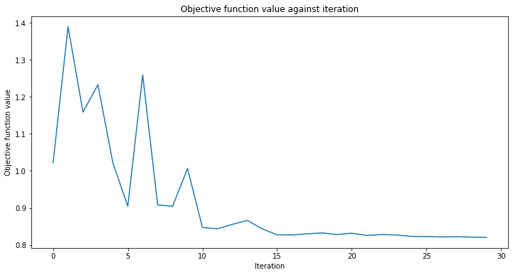
# create empty array for callback to store evaluations of the objective function
objective_func_vals = []
plt.rcParams["figure.figsize"] = (12, 6)

# fit classifier to data
sampler_classifier.fit(X, y01)

# return to default figsize
plt.rcParams["figure.figsize"] = (6, 4)

# score classifier
sampler_classifier.score(X, y01)
[15]:
0.7
[16]:
# evaluate data points
y_predict = sampler_classifier.predict(X)

# plot results
# red == wrongly classified
for x, y_target, y_p in zip(X, y01, y_predict):
    if y_target == 1:
        plt.plot(x[0], x[1], "bo")
    else:
        plt.plot(x[0], x[1], "go")
    if y_target != y_p:
        plt.scatter(x[0], x[1], s=200, facecolors="none", edgecolors="r", linewidths=2)
plt.plot([-1, 1], [1, -1], "--", color="black")
plt.show()
Encore une fois, une fois le modèle entraîné, nous pouvons examiner les poids. Comme nous avons défini ``reps=1``explicitement dans notre ansatz, nous pouvons voir moins de paramètres que dans le modèle précédent.
[17]:
sampler_classifier.weights
[17]:
array([ 1.67198565, 0.46045402, -0.93462862, -0.95266092])
Classifieur Variationnel Quantique (VQC)#
VQC est une variante spéciale de NeuralNetworkClassifier avec un SamplerQNN. Il applique une correspondance de parité (ou des extensions à plusieurs classes) pour mapper la chaîne de bits à la classification, ce qui donne lieu à un vecteur de probabilité, qui est interprété comme un résultat à encodage 1 parmi n (one-hot encoding). Par défaut, il applique la fonction CrossEntropyLoss qui attend les étiquettes données en un format d’encodage 1 parmi n et qui renverra également les prédictions dans ce format.
[18]:
# construct feature map, ansatz, and optimizer
feature_map = ZZFeatureMap(num_inputs)
ansatz = RealAmplitudes(num_inputs, reps=1)

# construct variational quantum classifier
vqc = VQC(
    feature_map=feature_map,
    ansatz=ansatz,
    loss="cross_entropy",
    optimizer=COBYLA(maxiter=30),
    callback=callback_graph,
)
[19]:
# create empty array for callback to store evaluations of the objective function
objective_func_vals = []
plt.rcParams["figure.figsize"] = (12, 6)

# fit classifier to data
vqc.fit(X, y_one_hot)

# return to default figsize
plt.rcParams["figure.figsize"] = (6, 4)

# score classifier
vqc.score(X, y_one_hot)
[19]:
0.8
[20]:
# evaluate data points
y_predict = vqc.predict(X)

# plot results
# red == wrongly classified
for x, y_target, y_p in zip(X, y_one_hot, y_predict):
    if y_target[0] == 1:
        plt.plot(x[0], x[1], "bo")
    else:
        plt.plot(x[0], x[1], "go")
    if not np.all(y_target == y_p):
        plt.scatter(x[0], x[1], s=200, facecolors="none", edgecolors="r", linewidths=2)
plt.plot([-1, 1], [1, -1], "--", color="black")
plt.show()
Classes multiples avec VQC#
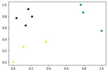
Dans cette section, nous générons un jeu de données artificiel contenant des échantillons de trois classes et montrant comment former un modèle pour classer ce jeu de données. Cet exemple montre comment résoudre des problèmes plus intéressants dans l’apprentissage automatique. Bien sûr, pour des raisons de durée d’entraînement, nous préparons un petit jeu de données. Nous utilisons make_classification de SciKit-Learn pour générer un jeu de données. Il y a 10 échantillons dans le jeu de données, 2 fonctionnalités, ce qui signifie que nous pouvons encore avoir un joli tracé du jeu de données, ainsi qu’aucune fonctionnalité redondante, ces fonctionnalités sont générées en tant que combinaisons des autres fonctionnalités. De plus, nous avons 3 classes différentes dans le jeu de données, chaque classe un type de centroid et nous définissons la séparation de classe à 2. ``, une légère augmentation à partir de la valeur par défaut de ``1.0 pour faciliter le problème de classification.
Une fois que le jeu de données est généré, nous mettons à l’échelle les fonctionnalités dans la plage [0, 1].
[21]:
from sklearn.datasets import make_classification
from sklearn.preprocessing import MinMaxScaler

X, y = make_classification(
    n_samples=10,
    n_features=2,
    n_classes=3,
    n_redundant=0,
    n_clusters_per_class=1,
    class_sep=2.0,
    random_state=algorithm_globals.random_seed,
)
X = MinMaxScaler().fit_transform(X)
Let’s see how our dataset looks like.
[22]:
plt.scatter(X[:, 0], X[:, 1], c=y)
[22]:
<matplotlib.collections.PathCollection at 0x7fd5e072c250>
We also transform labels and make them categorical.
[23]:
y_cat = np.empty(y.shape, dtype=str)
y_cat[y == 0] = "A"
y_cat[y == 1] = "B"
y_cat[y == 2] = "C"
print(y_cat)
['A' 'A' 'B' 'C' 'C' 'A' 'B' 'B' 'A' 'C']
We create an instance of VQC similar to the previous example, but in this case we pass a minimal set of parameters. Instead of feature map and ansatz we pass just the number of qubits that is equal to the number of features in the dataset, an optimizer with a low number of iteration to reduce training time, a quantum instance, and a callback to observe progress.
[24]:
vqc = VQC(
    num_qubits=2,
    optimizer=COBYLA(maxiter=30),
    callback=callback_graph,
)
Start the training process in the same way as in previous examples.
[25]:
# create empty array for callback to store evaluations of the objective function
objective_func_vals = []
plt.rcParams["figure.figsize"] = (12, 6)

# fit classifier to data
vqc.fit(X, y_cat)

# return to default figsize
plt.rcParams["figure.figsize"] = (6, 4)

# score classifier
vqc.score(X, y_cat)
[25]:
0.9
Despite we had the low number of iterations, we achieved quite a good score. Let see the output of the predict method and compare the output with the ground truth.
[26]:
predict = vqc.predict(X)
print(f"Predicted labels: {predict}")
print(f"Ground truth:     {y_cat}")
Predicted labels: ['A' 'A' 'B' 'C' 'C' 'A' 'B' 'B' 'A' 'B']
Ground truth:     ['A' 'A' 'B' 'C' 'C' 'A' 'B' 'B' 'A' 'C']
Régression#
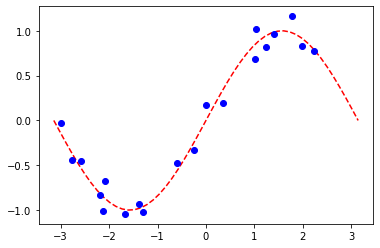
Nous préparons un ensemble de données de régression simple pour illustrer les algorithmes suivants.
[27]:
num_samples = 20
eps = 0.2
lb, ub = -np.pi, np.pi
X_ = np.linspace(lb, ub, num=50).reshape(50, 1)
f = lambda x: np.sin(x)

X = (ub - lb) * algorithm_globals.random.random([num_samples, 1]) + lb
y = f(X[:, 0]) + eps * (2 * algorithm_globals.random.random(num_samples) - 1)

plt.plot(X_, f(X_), "r--")
plt.plot(X, y, "bo")
plt.show()
Classification avec EstimatorQNN#
Here we restrict to regression with an EstimatorQNN that returns values in \([-1, +1]\). More complex and also multi-dimensional models could be constructed, also based on SamplerQNN but that exceeds the scope of this tutorial.
[28]:
# construct simple feature map
param_x = Parameter("x")
feature_map = QuantumCircuit(1, name="fm")
feature_map.ry(param_x, 0)

# construct simple ansatz
param_y = Parameter("y")
ansatz = QuantumCircuit(1, name="vf")
ansatz.ry(param_y, 0)

# construct a circuit
qc = QNNCircuit(feature_map=feature_map, ansatz=ansatz)

# construct QNN
regression_estimator_qnn = EstimatorQNN(circuit=qc)
[29]:
# construct the regressor from the neural network
regressor = NeuralNetworkRegressor(
    neural_network=regression_estimator_qnn,
    loss="squared_error",
    optimizer=L_BFGS_B(maxiter=5),
    callback=callback_graph,
)
[30]:
# create empty array for callback to store evaluations of the objective function
objective_func_vals = []
plt.rcParams["figure.figsize"] = (12, 6)

# fit to data
regressor.fit(X, y)

# return to default figsize
plt.rcParams["figure.figsize"] = (6, 4)

# score the result
regressor.score(X, y)
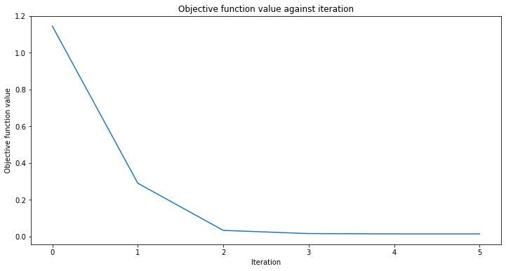
[30]:
0.9769994291935522
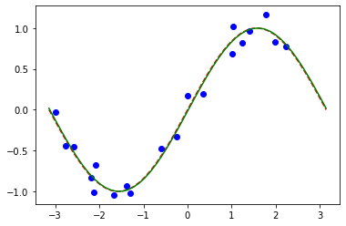
[31]:
# plot target function
plt.plot(X_, f(X_), "r--")

# plot data
plt.plot(X, y, "bo")

# plot fitted line
y_ = regressor.predict(X_)
plt.plot(X_, y_, "g-")
plt.show()
Similarly to the classification models, we can obtain an array of trained weights by querying a corresponding property of the model. In this model we have only one parameter defined as param_y above.
[32]:
regressor.weights
[32]:
array([-1.58870599])
Régression avec le Régresseur Quantique Variationnel (VQR)#
Similar to the VQC for classification, the VQR is a special variant of the NeuralNetworkRegressor with a EstimatorQNN. By default it considers the L2Loss function to minimize the mean squared error between predictions and targets.
[33]:
vqr = VQR(
    feature_map=feature_map,
    ansatz=ansatz,
    optimizer=L_BFGS_B(maxiter=5),
    callback=callback_graph,
)
[34]:
# create empty array for callback to store evaluations of the objective function
objective_func_vals = []
plt.rcParams["figure.figsize"] = (12, 6)

# fit regressor
vqr.fit(X, y)

# return to default figsize
plt.rcParams["figure.figsize"] = (6, 4)

# score result
vqr.score(X, y)
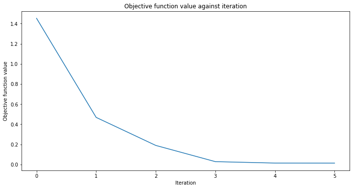
[34]:
0.9769955693935385
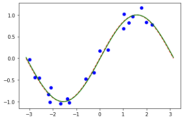
[35]:
# plot target function
plt.plot(X_, f(X_), "r--")

# plot data
plt.plot(X, y, "bo")

# plot fitted line
y_ = vqr.predict(X_)
plt.plot(X_, y_, "g-")
plt.show()
[36]:
import qiskit.tools.jupyter

%qiskit_version_table
%qiskit_copyright
Version Information
| Qiskit Software | Version |
|---|---|
qiskit-terra | 0.24.0 |
qiskit-aer | 0.12.0 |
qiskit-ignis | 0.6.0 |
qiskit-ibmq-provider | 0.20.2 |
qiskit | 0.43.0 |
qiskit-machine-learning | 0.7.0 |
| System information | |
| Python version | 3.8.8 |
| Python compiler | Clang 10.0.0 |
| Python build | default, Apr 13 2021 12:59:45 |
| OS | Darwin |
| CPUs | 8 |
| Memory (Gb) | 32.0 |
| Tue Jun 13 16:39:30 2023 CEST | |
This code is a part of Qiskit
© Copyright IBM 2017, 2023.
This code is licensed under the Apache License, Version 2.0. You may
obtain a copy of this license in the LICENSE.txt file in the root directory
of this source tree or at http://www.apache.org/licenses/LICENSE-2.0.
Any modifications or derivative works of this code must retain this
copyright notice, and modified files need to carry a notice indicating
that they have been altered from the originals.