Low-weight observables (Marginals)

Often one is interested in computing expectation values of “low-weight” observables, where the operator is comprised of one or more identity operators, e.g. \(\langle IIZZII\rangle\). Qubits with an idenitiy do not need to be corrected because the eigenvalues associated with the \(|0\rangle\) and \(|1\rangle\) states are the same. Because M3 scales with the number of bit-strings, removing these unneeded elements can reduce the amount of computation required. Below is an example of how to use M3 to marginalize and correct over the smaller distribution.

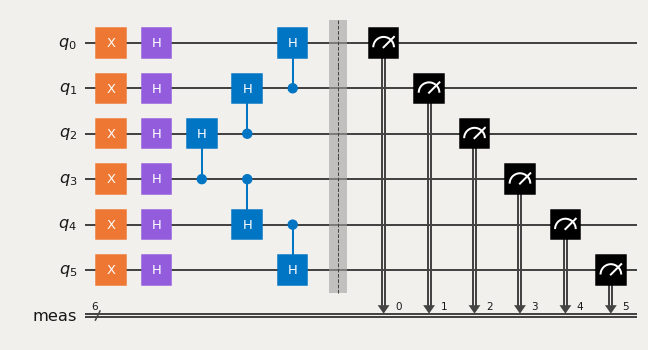
Consider the following circuit that we would like to evaluate:

from qiskit import *
from qiskit.providers.fake_provider import FakeGuadalupe
import mthree

N = 6
qc = QuantumCircuit(N)
qc.x(range(0, N))
qc.h(range(0, N))
for kk in range(N//2,0,-1):
    qc.ch(kk, kk-1)
for kk in range(N//2, N-1):
    qc.ch(kk, kk+1)
qc.measure_all()
qc.draw('mpl')

Let us first map this onto the target system and compute the final measurement mapping:

backend = FakeGuadalupe()

trans_qc = transpile(qc, backend, optimization_level=3, seed_transpiler=12345)
mapping = mthree.utils.final_measurement_mapping(trans_qc)
mapping

{0: 14, 1: 13, 2: 12, 3: 10, 4: 7, 5: 6}

Now assume we are only interested in many low-weight operators such as \(\langle ZIIZIZ\rangle\) or \(\langle ZZIIII\rangle\). How would we compute the corrected expectation values? Because there are identity operators, we can marginalize the distributions to be only over those qubits that actually play a role in the expectation value. However, we must remember to keep track of which physical qubits go to which classical bits. We can do this with mthree.utils.marginal_distribution():.

First let us first get a raw distribution:

counts = backend.run(trans_qc, shots=10000).result().get_counts()

We can get the marginal distributions in two ways. First we can directly pass a list of indices, e.g. for the operator \(\langle ZIIZIZ\rangle\) the list would be [0, 2, 5]:

mthree.utils.marginal_distribution(counts, [0, 2, 5])

{'100': 549,
 '011': 795,
 '001': 516,
 '110': 293,
 '000': 200,
 '111': 5955,
 '101': 1652,
 '010': 40}

or we can use the operator itself:

mthree.utils.marginal_distribution(counts, 'ZIIZIZ')

{'100': 549,
 '011': 795,
 '001': 516,
 '110': 293,
 '000': 200,
 '111': 5955,
 '101': 1652,
 '010': 40}

Now we have a marginal distribution and in principle we have enough. However, having a reduced mapping of physical qubits that correspond to the bits in the marginal distribution would be handy to have. We can pass a mapping to marginal_distribution and get such a reduced mapping:

marginal_counts, reduced_map = mthree.utils.marginal_distribution(counts, 'ZIIZIZ', mapping=mapping)
reduced_map

{0: 14, 1: 12, 2: 6}

We can now mitigate in a smaller probability space:

mit = mthree.M3Mitigation(backend)
mit.cals_from_system(reduced_map, shots=25000)

quasi = mit.apply_correction(marginal_counts, reduced_map)
quasi

{'000': 0.01701407673479919,
 '001': 0.04753294603460713,
 '010': 0.0007362968790037407,
 '011': 0.06997653514464955,
 '100': 0.04989385201099876,
 '101': 0.15528667734186424,
 '110': 0.00655644968471517,
 '111': 0.6530031661693623}

Because the only non-identity operators are typically Z operators it is easy to compute the eigenvalues because the operator will be all Z’s:

quasi.expval()

-0.5023325221879438