Note
This page was generated from docs/tutorials/09_application_classes.ipynb.
Application Classes for Optimization Problems#
Introduction#
We introduce application classes for the following optimization problems so that users can easily try various optimization problems on quantum computers.
Exact cover problem
Given a collection of subsets of items, find a subcollection such that each item is covered exactly once.
Knapsack problem
Given a set of items, find a subset of items such that the total weight is within the capacity and the total value is maximized.
Number partition problem
Given a multiset of positive integers, find a partition of the multiset into two subsets such that the sums of the subsets are equal.
Set packing problem
Given a collection of subsets of items, find a subcollection such that all subsets of the subcollection are pairwise disjoint and the number of items in the subcollection is maximized.
Graph problems
Clique problem
Given an undirected graph, find a subset of nodes with a specified number or the maximum number such that the induced subgraph is complete.
Graph partition problem
Given an undirected graph, find a partition into two components whose sizes are equal such that the total capacity of the edges between the two components is minimized.
Max-cut problem
Given an undirected graph, find a partition of nodes into two subsets such that the total weight of the edges between the two subsets is maximized.
Stable set problem
Given an undirected graph, find a subset of nodes such that no edge connects the nodes in the subset and the number of nodes is maximized.
Traveling salesman problem
Given a graph, find a route with the minimum distance such that the route visits each city exactly once.
Vehicle routing problem
Given a graph, a depot node, and the number of vehicles (routes), find a set of routes such that each node is covered exactly once except the depot and the total distance of the routes is minimized.
Vertex cover problem
Given an undirected graph, find a subset of nodes with the minimum size such that each edge has at least one endpoint in the subsets.
The application classes for graph problems (GraphOptimizationApplication) provide a functionality to draw graphs of an instance and a result. Note that you need to install matplotlib beforehand to utilize the functionality.
We introduce examples of the vertex cover problem and the knapsack problem in this page.
Examples of the max-cut problem and the traveling salesman problem are available in Max-Cut and Traveling Salesman Problem.
We first import packages necessary for application classes.
[1]:
from qiskit_optimization.algorithms import MinimumEigenOptimizer
from qiskit_algorithms.utils import algorithm_globals
from qiskit_algorithms import QAOA, NumPyMinimumEigensolver
from qiskit_algorithms.optimizers import COBYLA
from qiskit.primitives import Sampler
Vertex cover problem#
We introduce the application class for the vertex cover problem as an example of graph problems. Given an undirected graph, the vertex cover problem asks us to find a subset of nodes with the minimum size such that all edges are covered by any node selected.
We import the application class VertexCover for the vertex cover problem and networkx to generate a random graph.
[2]:
from qiskit_optimization.applications.vertex_cover import VertexCover
import networkx as nx

seed = 123
algorithm_globals.random_seed = seed
[3]:
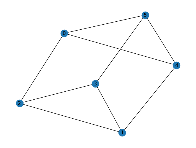
graph = nx.random_regular_graph(d=3, n=6, seed=seed)
pos = nx.spring_layout(graph, seed=seed)
[4]:
prob = VertexCover(graph)
prob.draw(pos=pos)
VertexCover takes a graph as an instance and to_quadratic_program generates a corresponding QuadraticProgram of the instance of the vertex cover problem.
[5]:
qp = prob.to_quadratic_program()
print(qp.prettyprint())
Problem name: Vertex cover

Minimize
  x_0 + x_1 + x_2 + x_3 + x_4 + x_5

Subject to
  Linear constraints (9)
    x_1 + x_2 >= 1  'c0'
    x_1 + x_4 >= 1  'c1'
    x_1 + x_3 >= 1  'c2'
    x_2 + x_3 >= 1  'c3'
    x_0 + x_2 >= 1  'c4'
    x_0 + x_4 >= 1  'c5'
    x_0 + x_5 >= 1  'c6'
    x_4 + x_5 >= 1  'c7'
    x_3 + x_5 >= 1  'c8'

  Binary variables (6)
    x_0 x_1 x_2 x_3 x_4 x_5
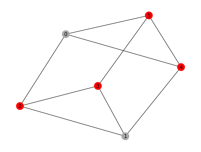
You can solve the problem as follows. NumPyMinimumEigensolver finds the minimum eigen vector. You can also apply QAOA. Note that the solution by QAOA is not always optimal.
[6]:
# Numpy Eigensolver
meo = MinimumEigenOptimizer(min_eigen_solver=NumPyMinimumEigensolver())
result = meo.solve(qp)
print(result.prettyprint())
print("\nsolution:", prob.interpret(result))
prob.draw(result, pos=pos)
objective function value: 4.0
variable values: x_0=0.0, x_1=0.0, x_2=1.0, x_3=1.0, x_4=1.0, x_5=1.0
status: SUCCESS

solution: [2, 3, 4, 5]
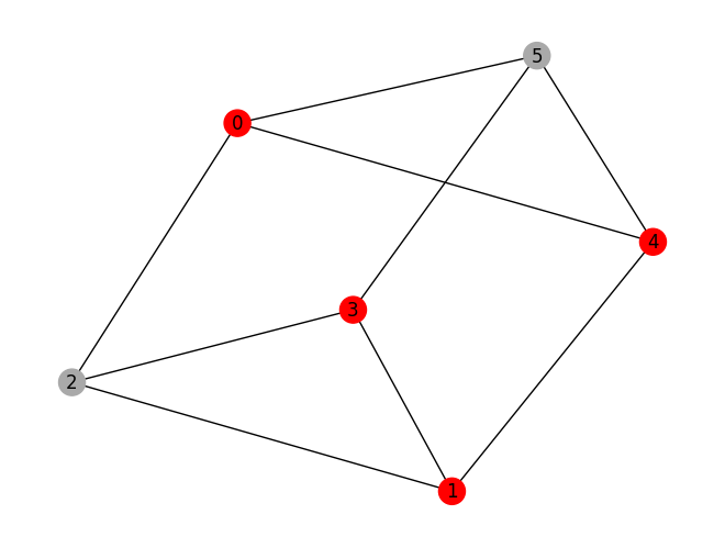
[7]:
# QAOA
meo = MinimumEigenOptimizer(min_eigen_solver=QAOA(reps=1, sampler=Sampler(), optimizer=COBYLA()))
result = meo.solve(qp)
print(result.prettyprint())
print("\nsolution:", prob.interpret(result))
print("\ntime:", result.min_eigen_solver_result.optimizer_time)
prob.draw(result, pos=pos)
objective function value: 4.0
variable values: x_0=1.0, x_1=1.0, x_2=0.0, x_3=1.0, x_4=1.0, x_5=0.0
status: SUCCESS

solution: [0, 1, 3, 4]

time: 1.5664818286895752
Knapsack problem#
The knapsack problem asks us to find a combination of items such that the total weight is within the capacity of the knapsack and maximize the total value of the items. The following examples solve an instance of the knapsack problem with 5 items by Numpy eigensolver and QAOA.
[8]:
from qiskit_optimization.applications import Knapsack
[9]:
prob = Knapsack(values=[3, 4, 5, 6, 7], weights=[2, 3, 4, 5, 6], max_weight=10)
qp = prob.to_quadratic_program()
print(qp.prettyprint())
Problem name: Knapsack

Maximize
  3*x_0 + 4*x_1 + 5*x_2 + 6*x_3 + 7*x_4

Subject to
  Linear constraints (1)
    2*x_0 + 3*x_1 + 4*x_2 + 5*x_3 + 6*x_4 <= 10  'c0'

  Binary variables (5)
    x_0 x_1 x_2 x_3 x_4
[10]:
# Numpy Eigensolver
meo = MinimumEigenOptimizer(min_eigen_solver=NumPyMinimumEigensolver())
result = meo.solve(qp)
print(result.prettyprint())
print("\nsolution:", prob.interpret(result))
objective function value: 13.0
variable values: x_0=1.0, x_1=1.0, x_2=0.0, x_3=1.0, x_4=0.0
status: SUCCESS

solution: [0, 1, 3]
[11]:
# QAOA
meo = MinimumEigenOptimizer(min_eigen_solver=QAOA(reps=1, sampler=Sampler(), optimizer=COBYLA()))
result = meo.solve(qp)
print(result.prettyprint())
print("\nsolution:", prob.interpret(result))
print("\ntime:", result.min_eigen_solver_result.optimizer_time)
objective function value: 13.0
variable values: x_0=1.0, x_1=1.0, x_2=0.0, x_3=1.0, x_4=0.0
status: SUCCESS

solution: [0, 1, 3]

time: 1.0938811302185059
How to check the Hamiltonian#
If you want to check the actual Hamiltonian generated from your problem instance, you need to apply a converter as follows.
[12]:
from qiskit_optimization.converters import QuadraticProgramToQubo
[13]:
# the same knapsack problem instance as in the previous section
prob = Knapsack(values=[3, 4, 5, 6, 7], weights=[2, 3, 4, 5, 6], max_weight=10)
qp = prob.to_quadratic_program()
print(qp.prettyprint())
Problem name: Knapsack

Maximize
  3*x_0 + 4*x_1 + 5*x_2 + 6*x_3 + 7*x_4

Subject to
  Linear constraints (1)
    2*x_0 + 3*x_1 + 4*x_2 + 5*x_3 + 6*x_4 <= 10  'c0'

  Binary variables (5)
    x_0 x_1 x_2 x_3 x_4
[14]:
# intermediate QUBO form of the optimization problem
conv = QuadraticProgramToQubo()
qubo = conv.convert(qp)
print(qubo.prettyprint())
Problem name: Knapsack

Minimize
  26*c0@int_slack@0^2 + 104*c0@int_slack@0*c0@int_slack@1
  + 208*c0@int_slack@0*c0@int_slack@2 + 156*c0@int_slack@0*c0@int_slack@3
  + 104*c0@int_slack@1^2 + 416*c0@int_slack@1*c0@int_slack@2
  + 312*c0@int_slack@1*c0@int_slack@3 + 416*c0@int_slack@2^2
  + 624*c0@int_slack@2*c0@int_slack@3 + 234*c0@int_slack@3^2
  + 104*x_0*c0@int_slack@0 + 208*x_0*c0@int_slack@1 + 416*x_0*c0@int_slack@2
  + 312*x_0*c0@int_slack@3 + 104*x_0^2 + 312*x_0*x_1 + 416*x_0*x_2 + 520*x_0*x_3
  + 624*x_0*x_4 + 156*x_1*c0@int_slack@0 + 312*x_1*c0@int_slack@1
  + 624*x_1*c0@int_slack@2 + 468*x_1*c0@int_slack@3 + 234*x_1^2 + 624*x_1*x_2
  + 780*x_1*x_3 + 936*x_1*x_4 + 208*x_2*c0@int_slack@0 + 416*x_2*c0@int_slack@1
  + 832*x_2*c0@int_slack@2 + 624*x_2*c0@int_slack@3 + 416*x_2^2 + 1040*x_2*x_3
  + 1248*x_2*x_4 + 260*x_3*c0@int_slack@0 + 520*x_3*c0@int_slack@1
  + 1040*x_3*c0@int_slack@2 + 780*x_3*c0@int_slack@3 + 650*x_3^2 + 1560*x_3*x_4
  + 312*x_4*c0@int_slack@0 + 624*x_4*c0@int_slack@1 + 1248*x_4*c0@int_slack@2
  + 936*x_4*c0@int_slack@3 + 936*x_4^2 - 520*c0@int_slack@0
  - 1040*c0@int_slack@1 - 2080*c0@int_slack@2 - 1560*c0@int_slack@3 - 1043*x_0
  - 1564*x_1 - 2085*x_2 - 2606*x_3 - 3127*x_4 + 2600

Subject to
  No constraints

  Binary variables (9)
    x_0 x_1 x_2 x_3 x_4 c0@int_slack@0 c0@int_slack@1 c0@int_slack@2
    c0@int_slack@3
[15]:
# qubit Hamiltonian and offset
op, offset = qubo.to_ising()
print(f"num qubits: {op.num_qubits}, offset: {offset}\n")
print(op)
num qubits: 9, offset: 1417.5

SparsePauliOp(['IIIIIIIIZ', 'IIIIIIIZI', 'IIIIIIZII', 'IIIIIZIII', 'IIIIZIIII', 'IIIZIIIII', 'IIZIIIIII', 'IZIIIIIII', 'ZIIIIIIII', 'IIIIIIIZZ', 'IIIIIIZIZ', 'IIIIIIZZI', 'IIIIIZIIZ', 'IIIIIZIZI', 'IIIIIZZII', 'IIIIZIIIZ', 'IIIIZIIZI', 'IIIIZIZII', 'IIIIZZIII', 'IIIZIIIIZ', 'IIIZIIIZI', 'IIIZIIZII', 'IIIZIZIII', 'IIIZZIIII', 'IIZIIIIIZ', 'IIZIIIIZI', 'IIZIIIZII', 'IIZIIZIII', 'IIZIZIIII', 'IIZZIIIII', 'IZIIIIIIZ', 'IZIIIIIZI', 'IZIIIIZII', 'IZIIIZIII', 'IZIIZIIII', 'IZIZIIIII', 'IZZIIIIII', 'ZIIIIIIIZ', 'ZIIIIIIZI', 'ZIIIIIZII', 'ZIIIIZIII', 'ZIIIZIIII', 'ZIIZIIIII', 'ZIZIIIIII', 'ZZIIIIIII'],
              coeffs=[-258.5+0.j, -388. +0.j, -517.5+0.j, -647. +0.j, -776.5+0.j, -130. +0.j,
 -260. +0.j, -520. +0.j, -390. +0.j,   78. +0.j,  104. +0.j,  156. +0.j,
  130. +0.j,  195. +0.j,  260. +0.j,  156. +0.j,  234. +0.j,  312. +0.j,
  390. +0.j,   26. +0.j,   39. +0.j,   52. +0.j,   65. +0.j,   78. +0.j,
   52. +0.j,   78. +0.j,  104. +0.j,  130. +0.j,  156. +0.j,   26. +0.j,
  104. +0.j,  156. +0.j,  208. +0.j,  260. +0.j,  312. +0.j,   52. +0.j,
  104. +0.j,   78. +0.j,  117. +0.j,  156. +0.j,  195. +0.j,  234. +0.j,
   39. +0.j,   78. +0.j,  156. +0.j])
[16]:
import tutorial_magics

%qiskit_version_table
%qiskit_copyright
Version Information
| Software | Version |
|---|---|
qiskit | 1.0.1 |
qiskit_optimization | 0.6.1 |
qiskit_algorithms | 0.3.0 |
| System information | |
| Python version | 3.8.18 |
| OS | Linux |
| Wed Feb 28 03:00:00 2024 UTC | |
This code is a part of a Qiskit project
© Copyright IBM 2017, 2024.
This code is licensed under the Apache License, Version 2.0. You may
obtain a copy of this license in the LICENSE.txt file in the root directory
of this source tree or at http://www.apache.org/licenses/LICENSE-2.0.
Any modifications or derivative works of this code must retain this
copyright notice, and modified files need to carry a notice indicating
that they have been altered from the originals.
[ ]: