注釈

このページは docs/tutorials/09_application_classes.ipynb から生成されました。

最適化問題のアプリケーション・クラス#

はじめに#

ユーザーが量子コンピューターで様々な最適化問題を簡単に試みることができるように、以下の最適化問題のアプリケーションクラスを導入します。

厳密被覆問題

アイテムのサブセットのコレクションが与えられた場合、それぞれのアイテムが正確に１回カバーされるような、サブコレクションを探します。

ナップサック問題

一連のアイテムを与えられた場合、合計重量が容量内にあり、合計値が最大化されるようなアイテムのサブセットを見つけます。

整数分割問題

正の整数のマルチセットが所与の時、合計が等しい 2 つのサブセットにする分割を探します。

集合パッキング問題

アイテムのサブセットのコレクションが所与の時、全てのサブセットが互いに素で、アイテム数が最大になるサブコレクションを探します。

グラフ問題

クリーク問題

無向グラフが与えられた場合、誘導部分グラフが完全になるような、特定の数または最大数のノードの部分集合を探します。

グラフ分割問題

無向グラフが与えられた場合、サイズが同じ２つのコンポーネントへの分割を探します。２つのコンポーネント間のエッジの合計容量は最小にします。

最大カット問題

無向グラフが所与の時、ノードの二つの部分集合への分割を探します。二つの部分集合のエッジの重みの合計は最大になるようにします。

安定集合問題

無向グラフが所与の時、以下のノードのサブセットを探します。サブセット中でエッジがノードに接続せず、ノード数が最大のサブセットです。

巡回セールスマン問題

グラフが所与の時、最小の距離のルートを探します。ルートは街を正確に一度訪れます。

車両ルーティング問題

グラフと倉庫ノードと車輌 (ルート) 数が所与の時、ルートのセットを探します。倉庫ノードを除くノードは厳密に一度カバーされ、ルートの合計距離は最小になるようにします。

頂点被覆問題

無向グラフが所与の時、それぞれのエッジが最低一つのエンドポイントを持つような、最小サイズのノードサブセットを探します。

グラフの問題のアプリケーション・クラス (GraphOptimizationApplication) は、インスタンスと結果のグラフを描画する機能を提供します。この機能を利用するには、あらかじめ matplotlib をインストールする必要があることに注意してください。

このページでは、頂点被覆問題とナップサック問題の例を紹介します。

最大カット問題と巡回セールスマン問題の例は Max-Cut and Traveling Salesman Problem にあります。

最初にアプリケーションクラスに必要なパッケージをインポートします。

[1]:

from qiskit_optimization.algorithms import MinimumEigenOptimizer
from qiskit_algorithms.utils import algorithm_globals
from qiskit_algorithms import QAOA, NumPyMinimumEigensolver
from qiskit_algorithms.optimizers import COBYLA
from qiskit.primitives import Sampler

頂点被覆問題#

グラフの問題の例として、頂点被覆問題のアプリケーションクラスを紹介します。頂点被覆問題では、無向グラフを所与として、選択されたノードによって全てのエッジがカバーされるような、最小サイズのノードサブセットを検索することを求められます。

頂点被覆問題のための VertexCover アプリケーションクラスと、ランダムグラフを生成するための networkx をインポートします。

[2]:

from qiskit_optimization.applications.vertex_cover import VertexCover
import networkx as nx

seed = 123
algorithm_globals.random_seed = seed

[3]:

graph = nx.random_regular_graph(d=3, n=6, seed=seed)
pos = nx.spring_layout(graph, seed=seed)

[4]:

prob = VertexCover(graph)
prob.draw(pos=pos)

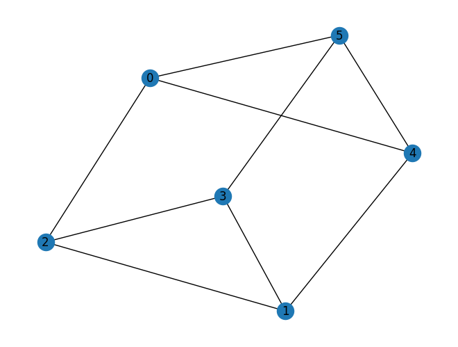
../_images/tutorials_09_application_classes_8_0.png

VertexCover はインスタンスとしてグラフを取り、to_quadratic_program は頂点被覆問題のインスタンスに対応する QuadraticProgram を生成します。

[5]:

qp = prob.to_quadratic_program()
print(qp.prettyprint())

Problem name: Vertex cover

Minimize
  x_0 + x_1 + x_2 + x_3 + x_4 + x_5

Subject to
  Linear constraints (9)
    x_1 + x_2 >= 1  'c0'
    x_1 + x_4 >= 1  'c1'
    x_1 + x_3 >= 1  'c2'
    x_2 + x_3 >= 1  'c3'
    x_0 + x_2 >= 1  'c4'
    x_0 + x_4 >= 1  'c5'
    x_0 + x_5 >= 1  'c6'
    x_4 + x_5 >= 1  'c7'
    x_3 + x_5 >= 1  'c8'

  Binary variables (6)
    x_0 x_1 x_2 x_3 x_4 x_5

この問題は以下のように解けます。NumPyMinimumEigensolver で最小固有ベクトルを見つけます。QAOA を適用しても良いです。ただし QAOA によるソリューションは常に最適ではないことに注意してください。

[6]:

# Numpy Eigensolver
meo = MinimumEigenOptimizer(min_eigen_solver=NumPyMinimumEigensolver())
result = meo.solve(qp)
print(result.prettyprint())
print("\nsolution:", prob.interpret(result))
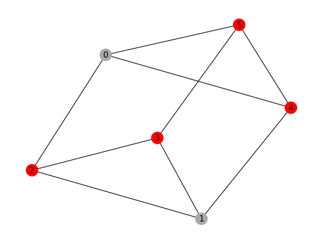
prob.draw(result, pos=pos)

objective function value: 4.0
variable values: x_0=0.0, x_1=0.0, x_2=1.0, x_3=1.0, x_4=1.0, x_5=1.0
status: SUCCESS

solution: [2, 3, 4, 5]

../_images/tutorials_09_application_classes_12_1.png

[7]:

# QAOA
meo = MinimumEigenOptimizer(min_eigen_solver=QAOA(reps=1, sampler=Sampler(), optimizer=COBYLA()))
result = meo.solve(qp)
print(result.prettyprint())
print("\nsolution:", prob.interpret(result))
print("\ntime:", result.min_eigen_solver_result.optimizer_time)
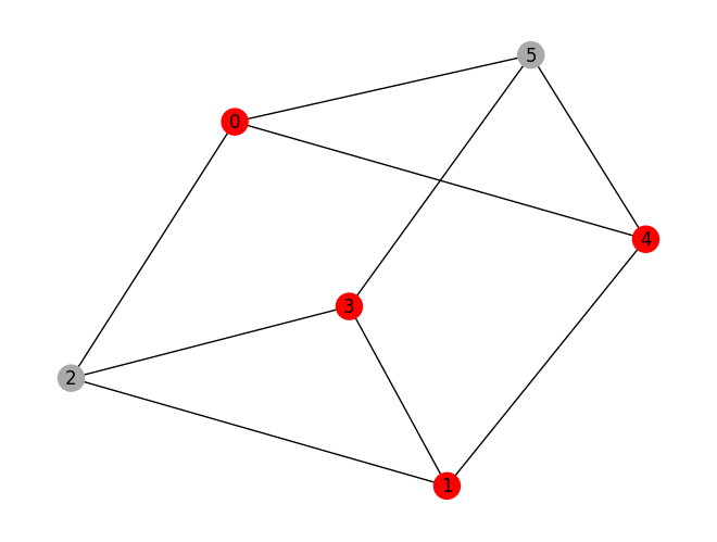
prob.draw(result, pos=pos)

objective function value: 4.0
variable values: x_0=1.0, x_1=1.0, x_2=0.0, x_3=1.0, x_4=1.0, x_5=0.0
status: SUCCESS

solution: [0, 1, 3, 4]

time: 2.721126079559326

../_images/tutorials_09_application_classes_13_1.png

ナップサック問題#

ナップサック問題は、総重量がナップサックの容量以下で、アイテムの総価値が最大になるアイテムの組合せを見つける問題です。以下の例では、Numpy eigensolver と QAOA によって、5 アイテムのナップサック問題の例を解きます。

[8]:

from qiskit_optimization.applications import Knapsack

[9]:

prob = Knapsack(values=[3, 4, 5, 6, 7], weights=[2, 3, 4, 5, 6], max_weight=10)
qp = prob.to_quadratic_program()
print(qp.prettyprint())

Problem name: Knapsack

Maximize
  3*x_0 + 4*x_1 + 5*x_2 + 6*x_3 + 7*x_4

Subject to
  Linear constraints (1)
    2*x_0 + 3*x_1 + 4*x_2 + 5*x_3 + 6*x_4 <= 10  'c0'

  Binary variables (5)
    x_0 x_1 x_2 x_3 x_4

[10]:

# Numpy Eigensolver
meo = MinimumEigenOptimizer(min_eigen_solver=NumPyMinimumEigensolver())
result = meo.solve(qp)
print(result.prettyprint())
print("\nsolution:", prob.interpret(result))

objective function value: 13.0
variable values: x_0=1.0, x_1=1.0, x_2=0.0, x_3=1.0, x_4=0.0
status: SUCCESS

solution: [0, 1, 3]

[11]:

# QAOA
meo = MinimumEigenOptimizer(min_eigen_solver=QAOA(reps=1, sampler=Sampler(), optimizer=COBYLA()))
result = meo.solve(qp)
print(result.prettyprint())
print("\nsolution:", prob.interpret(result))
print("\ntime:", result.min_eigen_solver_result.optimizer_time)

objective function value: 13.0
variable values: x_0=1.0, x_1=1.0, x_2=0.0, x_3=1.0, x_4=0.0
status: SUCCESS

solution: [0, 1, 3]

time: 2.0846190452575684

ハミルトニアンの確認方法#

問題インスタンスから生成された実際のハミルトニアンを確認するには、次のようにコンバーターを適用する必要があります。

[12]:

from qiskit_optimization.converters import QuadraticProgramToQubo

[13]:

# the same knapsack problem instance as in the previous section
prob = Knapsack(values=[3, 4, 5, 6, 7], weights=[2, 3, 4, 5, 6], max_weight=10)
qp = prob.to_quadratic_program()
print(qp.prettyprint())

Problem name: Knapsack

Maximize
  3*x_0 + 4*x_1 + 5*x_2 + 6*x_3 + 7*x_4

Subject to
  Linear constraints (1)
    2*x_0 + 3*x_1 + 4*x_2 + 5*x_3 + 6*x_4 <= 10  'c0'

  Binary variables (5)
    x_0 x_1 x_2 x_3 x_4

[14]:

# intermediate QUBO form of the optimization problem
conv = QuadraticProgramToQubo()
qubo = conv.convert(qp)
print(qubo.prettyprint())

Problem name: Knapsack

Minimize
  26*c0@int_slack@0^2 + 104*c0@int_slack@0*c0@int_slack@1
  + 208*c0@int_slack@0*c0@int_slack@2 + 156*c0@int_slack@0*c0@int_slack@3
  + 104*c0@int_slack@1^2 + 416*c0@int_slack@1*c0@int_slack@2
  + 312*c0@int_slack@1*c0@int_slack@3 + 416*c0@int_slack@2^2
  + 624*c0@int_slack@2*c0@int_slack@3 + 234*c0@int_slack@3^2
  + 104*x_0*c0@int_slack@0 + 208*x_0*c0@int_slack@1 + 416*x_0*c0@int_slack@2
  + 312*x_0*c0@int_slack@3 + 104*x_0^2 + 312*x_0*x_1 + 416*x_0*x_2 + 520*x_0*x_3
  + 624*x_0*x_4 + 156*x_1*c0@int_slack@0 + 312*x_1*c0@int_slack@1
  + 624*x_1*c0@int_slack@2 + 468*x_1*c0@int_slack@3 + 234*x_1^2 + 624*x_1*x_2
  + 780*x_1*x_3 + 936*x_1*x_4 + 208*x_2*c0@int_slack@0 + 416*x_2*c0@int_slack@1
  + 832*x_2*c0@int_slack@2 + 624*x_2*c0@int_slack@3 + 416*x_2^2 + 1040*x_2*x_3
  + 1248*x_2*x_4 + 260*x_3*c0@int_slack@0 + 520*x_3*c0@int_slack@1
  + 1040*x_3*c0@int_slack@2 + 780*x_3*c0@int_slack@3 + 650*x_3^2 + 1560*x_3*x_4
  + 312*x_4*c0@int_slack@0 + 624*x_4*c0@int_slack@1 + 1248*x_4*c0@int_slack@2
  + 936*x_4*c0@int_slack@3 + 936*x_4^2 - 520*c0@int_slack@0
  - 1040*c0@int_slack@1 - 2080*c0@int_slack@2 - 1560*c0@int_slack@3 - 1043*x_0
  - 1564*x_1 - 2085*x_2 - 2606*x_3 - 3127*x_4 + 2600

Subject to
  No constraints

  Binary variables (9)
    x_0 x_1 x_2 x_3 x_4 c0@int_slack@0 c0@int_slack@1 c0@int_slack@2
    c0@int_slack@3

[15]:

# qubit Hamiltonian and offset
op, offset = qubo.to_ising()
print(f"num qubits: {op.num_qubits}, offset: {offset}\n")
print(op)

num qubits: 9, offset: 1417.5

SparsePauliOp(['IIIIIIIIZ', 'IIIIIIIZI', 'IIIIIIZII', 'IIIIIZIII', 'IIIIZIIII', 'IIIZIIIII', 'IIZIIIIII', 'IZIIIIIII', 'ZIIIIIIII', 'IIIIIIIZZ', 'IIIIIIZIZ', 'IIIIIIZZI', 'IIIIIZIIZ', 'IIIIIZIZI', 'IIIIIZZII', 'IIIIZIIIZ', 'IIIIZIIZI', 'IIIIZIZII', 'IIIIZZIII', 'IIIZIIIIZ', 'IIIZIIIZI', 'IIIZIIZII', 'IIIZIZIII', 'IIIZZIIII', 'IIZIIIIIZ', 'IIZIIIIZI', 'IIZIIIZII', 'IIZIIZIII', 'IIZIZIIII', 'IIZZIIIII', 'IZIIIIIIZ', 'IZIIIIIZI', 'IZIIIIZII', 'IZIIIZIII', 'IZIIZIIII', 'IZIZIIIII', 'IZZIIIIII', 'ZIIIIIIIZ', 'ZIIIIIIZI', 'ZIIIIIZII', 'ZIIIIZIII', 'ZIIIZIIII', 'ZIIZIIIII', 'ZIZIIIIII', 'ZZIIIIIII'],
              coeffs=[-258.5+0.j, -388. +0.j, -517.5+0.j, -647. +0.j, -776.5+0.j, -130. +0.j,
 -260. +0.j, -520. +0.j, -390. +0.j,   78. +0.j,  104. +0.j,  156. +0.j,
  130. +0.j,  195. +0.j,  260. +0.j,  156. +0.j,  234. +0.j,  312. +0.j,
  390. +0.j,   26. +0.j,   39. +0.j,   52. +0.j,   65. +0.j,   78. +0.j,
   52. +0.j,   78. +0.j,  104. +0.j,  130. +0.j,  156. +0.j,   26. +0.j,
  104. +0.j,  156. +0.j,  208. +0.j,  260. +0.j,  312. +0.j,   52. +0.j,
  104. +0.j,   78. +0.j,  117. +0.j,  156. +0.j,  195. +0.j,  234. +0.j,
   39. +0.j,   78. +0.j,  156. +0.j])

[16]:

import qiskit.tools.jupyter

%qiskit_version_table
%qiskit_copyright

Version Information

Qiskit Software	Version
`qiskit-terra`	0.25.0.dev0+1d844ec
`qiskit-aer`	0.12.0
`qiskit-ibmq-provider`	0.20.2
`qiskit-nature`	0.7.0
`qiskit-optimization`	0.6.0
System information
Python version	3.10.11
Python compiler	Clang 14.0.0 (clang-1400.0.29.202)
Python build	main, Apr 7 2023 07:31:31
OS	Darwin
CPUs	4
Memory (Gb)	16.0
Thu May 18 16:57:10 2023 JST

This code is a part of Qiskit

This code is licensed under the Apache License, Version 2.0. You may
obtain a copy of this license in the LICENSE.txt file in the root directory
of this source tree or at http://www.apache.org/licenses/LICENSE-2.0.

Any modifications or derivative works of this code must retain this
copyright notice, and modified files need to carry a notice indicating
that they have been altered from the originals.

[ ]: