Nota
Esta página fue generada a partir de docs/tutorials/08_cvar_optimization.ipynb.
Mejora de la Optimización Cuántica Variacional mediante CVaR#
Introducción#
Este cuaderno muestra cómo utilizar la función objetivo de Valor en Riesgo Condicional (Conditional Value at Risk, CVaR) introducida en [1] dentro de los algoritmos de optimización cuántica variacional proporcionados por Qiskit Algorithms. En particular, se muestra cómo configurar el MinimumEigenOptimizer usando SamplingVQE como corresponde. Para un conjunto dado de iteraciones con los valores objetivos correspondientes al problema de optimización considerado, el CVaR con nivel de confianza \(\alpha \in [0, 1]\) se define como el promedio de las mejores iteraciones \(\alpha\). Por lo tanto, \(\alpha = 1\) corresponde al valor esperado estándar, mientras que \(\alpha=0\) corresponde al mínimo de las iteraciones realizadas, y \(\alpha \in (0, 1)\) es una compensación entre enfocarse en mejores iteraciones, pero aún así aplicar algunos promedios para suavizar el panorama de optimización.
Referencias#
[1] P. Barkoutsos et al., Improving Variational Quantum Optimization using CVaR, Quantum 4, 256 (2020).
[1]:
from qiskit.circuit.library import RealAmplitudes
from qiskit_algorithms.optimizers import COBYLA
from qiskit_algorithms import NumPyMinimumEigensolver, SamplingVQE
from qiskit_algorithms.utils import algorithm_globals
from qiskit.primitives import Sampler
from qiskit_optimization.converters import LinearEqualityToPenalty
from qiskit_optimization.algorithms import MinimumEigenOptimizer
from qiskit_optimization.translators import from_docplex_mp

import numpy as np
import matplotlib.pyplot as plt
from docplex.mp.model import Model
[2]:
algorithm_globals.random_seed = 123456
Optimización de Cartera#
A continuación, definimos una instancia del problema para la optimización de cartera como se presenta en [1].
[3]:
# prepare problem instance
n = 6  # number of assets
q = 0.5  # risk factor
budget = n // 2  # budget
penalty = 2 * n  # scaling of penalty term
[4]:
# instance from [1]
mu = np.array([0.7313, 0.9893, 0.2725, 0.8750, 0.7667, 0.3622])
sigma = np.array(
    [
        [0.7312, -0.6233, 0.4689, -0.5452, -0.0082, -0.3809],
        [-0.6233, 2.4732, -0.7538, 2.4659, -0.0733, 0.8945],
        [0.4689, -0.7538, 1.1543, -1.4095, 0.0007, -0.4301],
        [-0.5452, 2.4659, -1.4095, 3.5067, 0.2012, 1.0922],
        [-0.0082, -0.0733, 0.0007, 0.2012, 0.6231, 0.1509],
        [-0.3809, 0.8945, -0.4301, 1.0922, 0.1509, 0.8992],
    ]
)

# or create random instance
# mu, sigma = portfolio.random_model(n, seed=123)  # expected returns and covariance matrix
[5]:
# create docplex model
mdl = Model("portfolio_optimization")
x = mdl.binary_var_list(range(n), name="x")
objective = mdl.sum([mu[i] * x[i] for i in range(n)])
objective -= q * mdl.sum([sigma[i, j] * x[i] * x[j] for i in range(n) for j in range(n)])
mdl.maximize(objective)
mdl.add_constraint(mdl.sum(x[i] for i in range(n)) == budget)

# case to
qp = from_docplex_mp(mdl)
[6]:
# solve classically as reference
opt_result = MinimumEigenOptimizer(NumPyMinimumEigensolver()).solve(qp)
print(opt_result.prettyprint())
objective function value: 1.27835
variable values: x_0=1.0, x_1=1.0, x_2=0.0, x_3=0.0, x_4=1.0, x_5=0.0
status: SUCCESS
[7]:
# we convert the problem to an unconstrained problem for further analysis,
# otherwise this would not be necessary as the MinimumEigenSolver would do this
# translation automatically
linear2penalty = LinearEqualityToPenalty(penalty=penalty)
qp = linear2penalty.convert(qp)
_, offset = qp.to_ising()
Optimizador Propio Mínimo usando SamplingVQE#
[8]:
# set classical optimizer
maxiter = 100
optimizer = COBYLA(maxiter=maxiter)

# set variational ansatz
ansatz = RealAmplitudes(n, reps=1)
m = ansatz.num_parameters

# set sampler
sampler = Sampler()

# run variational optimization for different values of alpha
alphas = [1.0, 0.50, 0.25]  # confidence levels to be evaluated
[9]:
# dictionaries to store optimization progress and results
objectives = {alpha: [] for alpha in alphas}  # set of tested objective functions w.r.t. alpha
results = {}  # results of minimum eigensolver w.r.t alpha

# callback to store intermediate results
def callback(i, params, obj, stddev, alpha):
    # we translate the objective from the internal Ising representation
    # to the original optimization problem
    objectives[alpha].append(np.real_if_close(-(obj + offset)))


# loop over all given alpha values
for alpha in alphas:

    # initialize SamplingVQE using CVaR
    vqe = SamplingVQE(
        sampler=sampler,
        ansatz=ansatz,
        optimizer=optimizer,
        aggregation=alpha,
        callback=lambda i, params, obj, stddev: callback(i, params, obj, stddev, alpha),
    )

    # initialize optimization algorithm based on CVaR-SamplingVQE
    opt_alg = MinimumEigenOptimizer(vqe)

    # solve problem
    results[alpha] = opt_alg.solve(qp)

    # print results
    print("alpha = {}:".format(alpha))
    print(results[alpha].prettyprint())
    print()
alpha = 1.0:
objective function value: 1.2783500000000174
variable values: x_0=1.0, x_1=1.0, x_2=0.0, x_3=0.0, x_4=1.0, x_5=0.0
status: SUCCESS

alpha = 0.5:
objective function value: 1.2783500000000174
variable values: x_0=1.0, x_1=1.0, x_2=0.0, x_3=0.0, x_4=1.0, x_5=0.0
status: SUCCESS

alpha = 0.25:
objective function value: 1.2783500000000174
variable values: x_0=1.0, x_1=1.0, x_2=0.0, x_3=0.0, x_4=1.0, x_5=0.0
status: SUCCESS
[10]:
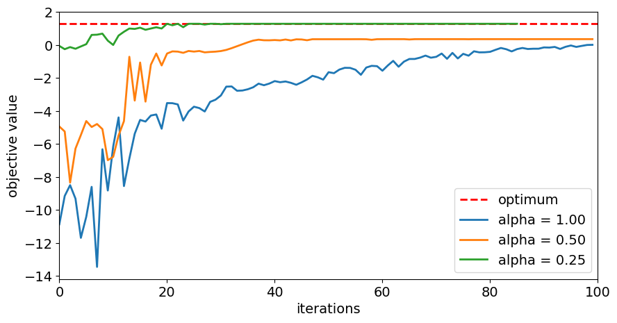
# plot resulting history of objective values
plt.figure(figsize=(10, 5))
plt.plot([0, maxiter], [opt_result.fval, opt_result.fval], "r--", linewidth=2, label="optimum")
for alpha in alphas:
    plt.plot(objectives[alpha], label="alpha = %.2f" % alpha, linewidth=2)
plt.legend(loc="lower right", fontsize=14)
plt.xlim(0, maxiter)
plt.xticks(fontsize=14)
plt.xlabel("iterations", fontsize=14)
plt.yticks(fontsize=14)
plt.ylabel("objective value", fontsize=14)
plt.show()
[11]:
# evaluate and sort all objective values
objective_values = np.zeros(2**n)
for i in range(2**n):
    x_bin = ("{0:0%sb}" % n).format(i)
    x = [0 if x_ == "0" else 1 for x_ in reversed(x_bin)]
    objective_values[i] = qp.objective.evaluate(x)
ind = np.argsort(objective_values)

# evaluate final optimal probability for each alpha
for alpha in alphas:
    probabilities = np.fromiter(
        results[alpha].min_eigen_solver_result.eigenstate.binary_probabilities().values(),
        dtype=float,
    )
    print("optimal probability (alpha = %.2f):  %.4f" % (alpha, probabilities[ind][-1:]))
optimal probability (alpha = 1.00):  0.0000
optimal probability (alpha = 0.50):  0.0000
optimal probability (alpha = 0.25):  0.2895
[12]:
import qiskit.tools.jupyter

%qiskit_version_table
%qiskit_copyright
Version Information
| Qiskit Software | Version |
|---|---|
qiskit-terra | 0.25.0.dev0+1d844ec |
qiskit-aer | 0.12.0 |
qiskit-ibmq-provider | 0.20.2 |
qiskit-nature | 0.7.0 |
qiskit-optimization | 0.6.0 |
| System information | |
| Python version | 3.10.11 |
| Python compiler | Clang 14.0.0 (clang-1400.0.29.202) |
| Python build | main, Apr 7 2023 07:31:31 |
| OS | Darwin |
| CPUs | 4 |
| Memory (Gb) | 16.0 |
| Thu May 18 16:56:49 2023 JST | |
This code is a part of Qiskit
© Copyright IBM 2017, 2023.
This code is licensed under the Apache License, Version 2.0. You may
obtain a copy of this license in the LICENSE.txt file in the root directory
of this source tree or at http://www.apache.org/licenses/LICENSE-2.0.
Any modifications or derivative works of this code must retain this
copyright notice, and modified files need to carry a notice indicating
that they have been altered from the originals.
[ ]: