নোট
এই পৃষ্ঠাটি docs/tutorials/07_leveraging_qiskit_runtime.ipynb থেকে বানানো হয়েছে।
Qiskit রানটাইম লিভারেজিং#
সতর্কতা
The VQEClient discussed in this tutorial is DEPRECATED as of version 0.6 of Qiskit Nature and will be removed no sooner than 3 months after the release. Instead you should use the new primitives based VQE with the Qiskit IBM Runtime Estimator primitive. For more details on how to migrate check out this guide here.
Iterative algorithms, such as the Variational Quantum Eigensolver (VQE), traditionally send one batch of circuits (one "job") to be executed on the quantum device in each iteration. Sending a job involves certain overhead, mainly
অনুরোধগুলি প্রক্রিয়া করার এবং ডেটা পাঠানোর সময় (API ওভারহেড, সাধারণত প্রায় 10s)
the job queue time, that is how long you have to wait before it’s your turn to run on the device (usually about 2min)
If we send hundreds of jobs iteratively, this overhead quickly dominates the execution time of our algorithm. Qiskit Runtime allows us to tackle these issues and significantly speed up (especially) iterative algorithms. With Qiskit Runtime, one job does not contain only a batch of circuits but the entire algorithm. That means we only experience the API overhead and queue wait once instead of in every iteration! You’ll be able to either upload algorithm parameters and delegate all the complexity to the cloud, where your program is executed, or upload your personal algorithm directly.
For the VQE, the integration of Qiskit Runtime in your existing code is a piece of cake. There is a (almost) drop-in replacement, called VQEClient for the VQE class.
Let’s see how you can leverage the runtime on a simple chemistry example: Finding the ground state energy of the lithium hydrate (LiH) molecule at a given bond distance.
সমস্যা স্পেসিফিকেশন: LiH অণু#
প্রথমত, আমরা অণু নির্দিষ্ট করি যার গ্রাউন্ড স্টেট এনার্জি আমরা চাই। এখানে, আমরা 2.5Å বন্ড দূরত্বের LiH এর দিকে তাকাই।
[1]:
from qiskit_nature.units import DistanceUnit
from qiskit_nature.second_q.drivers import PySCFDriver
from qiskit_nature.second_q.mappers import ParityMapper
from qiskit_nature.second_q.properties import ParticleNumber
from qiskit_nature.second_q.transformers import ActiveSpaceTransformer
[2]:
bond_distance = 2.5  # in Angstrom

# specify driver
driver = PySCFDriver(
    atom=f"Li 0 0 0; H 0 0 {bond_distance}",
    basis="sto3g",
    charge=0,
    spin=0,
    unit=DistanceUnit.ANGSTROM,
)
problem = driver.run()

# specify active space transformation
active_space_trafo = ActiveSpaceTransformer(
    num_electrons=problem.num_particles, num_spatial_orbitals=3
)

# transform the electronic structure problem
problem = active_space_trafo.transform(problem)

# construct the parity mapper with 2-qubit reduction
qubit_mapper = ParityMapper(num_particles=problem.num_particles)
প্রথাগত (ক্লাসিক্যাল) রেফারেন্স সমাধান#
একটি রেফারেন্স সমাধান হিসাবে আমরা NumPyEigensolver দিয়ে ক্লাসিকভাবে এই সিস্টেমটি সমাধান করতে পারি।
[3]:
from qiskit_algorithms import NumPyMinimumEigensolver
from qiskit_nature.second_q.algorithms.ground_state_solvers import GroundStateEigensolver

np_solver = NumPyMinimumEigensolver()
np_groundstate_solver = GroundStateEigensolver(qubit_mapper, np_solver)

np_result = np_groundstate_solver.solve(problem)
[19]:
target_energy = np_result.total_energies[0]
print(np_result)
=== GROUND STATE ENERGY ===

* Electronic ground state energy (Hartree): -8.408630641972
  - computed part:      -8.408630641972
  - ActiveSpaceTransformer extracted energy part: 0.0
~ Nuclear repulsion energy (Hartree): 0.635012653104
> Total ground state energy (Hartree): -7.773617988868

=== MEASURED OBSERVABLES ===

  0:  # Particles: 4.000 S: 0.000 S^2: 0.000 M: 0.000

=== DIPOLE MOMENTS ===

~ Nuclear dipole moment (a.u.): [0.0  0.0  4.72431531]

  0:
  * Electronic dipole moment (a.u.): [0.0  0.0  6.45025807]
    - computed part:      [0.0  0.0  6.45025807]
    - ActiveSpaceTransformer extracted energy part: [0.0  0.0  0.0]
  > Dipole moment (a.u.): [0.0  0.0  -1.72594276]  Total: 1.72594276
                 (debye): [0.0  0.0  -4.38690851]  Total: 4.38690851
ভি কিউ ই#
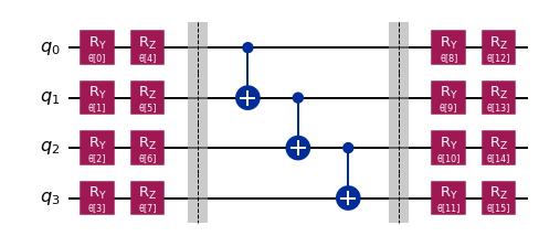
To run the VQE we need to select a parameterized quantum circuit acting as ansatz and a classical optimizer. Here we’ll choose a heuristic, hardware efficient ansatz and the SPSA optimizer.
[5]:
from qiskit.circuit.library import EfficientSU2

ansatz = EfficientSU2(num_qubits=4, reps=1, entanglement="linear", insert_barriers=True)
ansatz.decompose().draw("mpl", style="iqx")
[5]:
[6]:
import numpy as np
from qiskit.utils import algorithm_globals

# fix random seeds for reproducibility

np.random.seed(5)
algorithm_globals.random_seed = 5
[7]:
from qiskit_algorithms.optimizers import SPSA

optimizer = SPSA(maxiter=100)

initial_point = np.random.random(ansatz.num_parameters)
Before executing the VQE in the cloud using Qiskit Runtime, let’s execute a local VQE first.
[8]:
from qiskit_algorithms import VQE
from qiskit.primitives import Estimator

estimator = Estimator()

local_vqe = VQE(
    estimator,
    ansatz,
    optimizer,
    initial_point=initial_point,
)

local_vqe_groundstate_solver = GroundStateEigensolver(qubit_mapper, local_vqe)

local_vqe_result = local_vqe_groundstate_solver.solve(problem)
[9]:
print(local_vqe_result)
=== GROUND STATE ENERGY ===

* Electronic ground state energy (Hartree): -8.223473551005
  - computed part:      -8.223473551005
  - ActiveSpaceTransformer extracted energy part: 0.0
~ Nuclear repulsion energy (Hartree): 0.635012653104
> Total ground state energy (Hartree): -7.588460897901

=== MEASURED OBSERVABLES ===

  0:  # Particles: 3.997 S: 0.438 S^2: 0.631 M: 0.001

=== DIPOLE MOMENTS ===

~ Nuclear dipole moment (a.u.): [0.0  0.0  4.72431531]

  0:
  * Electronic dipole moment (a.u.): [0.0  0.0  1.41136787]
    - computed part:      [0.0  0.0  1.41136787]
    - ActiveSpaceTransformer extracted energy part: [0.0  0.0  0.0]
  > Dipole moment (a.u.): [0.0  0.0  3.31294744]  Total: 3.31294744
                 (debye): [0.0  0.0  8.42067168]  Total: 8.42067168
রানটাইম VQE#
Let’s exchange the eigensolver from a local VQE algorithm to a VQE executed using Qiskit Runtime – simply by exchanging the VQE class by the qiskit_nature.runtime.VQEClient.
First, we’ll have to load a provider to access Qiskit Runtime. Note: You have to replace the next cell with your provider.
[10]:
from qiskit import IBMQ

IBMQ.load_account()
provider = IBMQ.get_provider(group="open")  # replace by your runtime provider

backend = provider.get_backend("ibmq_qasm_simulator")  # select a backend that supports the runtime
Now we can set up the VQEClient. In this first release, the optimizer must be provided as a dictionary, in future releases you’ll be able to pass the same optimizer object as in the traditional VQE.
[11]:
from qiskit_nature.runtime import VQEClient

runtime_vqe = VQEClient(
    ansatz=ansatz,
    optimizer=optimizer,
    initial_point=initial_point,
    provider=provider,
    backend=backend,
    shots=1024,
    measurement_error_mitigation=True,
)  # use a complete measurement fitter for error mitigation
[12]:
runtime_vqe_groundstate_solver = GroundStateEigensolver(qubit_mapper, runtime_vqe)
runtime_vqe_result = runtime_vqe_groundstate_solver.solve(problem)
[13]:
print(runtime_vqe_result)
=== GROUND STATE ENERGY ===

* Electronic ground state energy (Hartree): -8.172591259069
  - computed part:      -8.172591259069
  - ActiveSpaceTransformer extracted energy part: 0.0
~ Nuclear repulsion energy (Hartree): 0.635012653104
> Total ground state energy (Hartree): -7.537578605965

=== MEASURED OBSERVABLES ===

  0:  # Particles: 3.988 S: 0.596 S^2: 0.951 M: 0.002

=== DIPOLE MOMENTS ===

~ Nuclear dipole moment (a.u.): [0.0  0.0  4.72431531]

  0:
  * Electronic dipole moment (a.u.): [0.0  0.0  1.25645131]
    - computed part:      [0.0  0.0  1.25645131]
    - ActiveSpaceTransformer extracted energy part: [0.0  0.0  0.0]
  > Dipole moment (a.u.): [0.0  0.0  3.467864]  Total: 3.467864
                 (debye): [0.0  0.0  8.81443024]  Total: 8.81443024
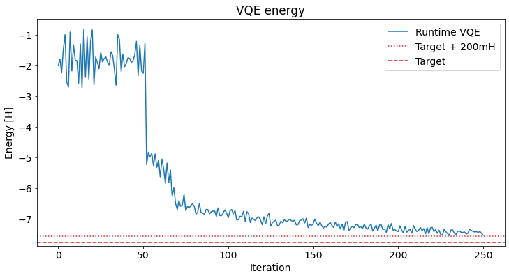
If we are interested in the development of the energy, the VQEClient allows access to the history of the optimizer, which contains the loss per iteration (along with the parameters and a timestamp). Note that this only holds for the SPSA and QN-SPSA optimizers. Otherwise you have to use a callback to the VQEClient, similar to the normal VQE.
We can access this data via the raw_result attribute of the ground state solver.
[17]:
runtime_result = runtime_vqe_result.raw_result
history = runtime_result.optimizer_history
loss = history["energy"]
[20]:
import matplotlib.pyplot as plt

plt.rcParams["font.size"] = 14

# plot loss and reference value
plt.figure(figsize=(12, 6))
plt.plot(loss + runtime_vqe_result.nuclear_repulsion_energy, label="Runtime VQE")
plt.axhline(y=target_energy + 0.2, color="tab:red", ls=":", label="Target + 200mH")
plt.axhline(y=target_energy, color="tab:red", ls="--", label="Target")

plt.legend(loc="best")
plt.xlabel("Iteration")
plt.ylabel("Energy [H]")
plt.title("VQE energy");
[21]:
import qiskit.tools.jupyter

%qiskit_version_table
%qiskit_copyright
Version Information
| Qiskit Software | Version |
|---|---|
qiskit-terra | 0.23.0.dev0+f339f71 |
qiskit-aer | 0.11.1 |
qiskit-ibmq-provider | 0.19.2 |
qiskit-nature | 0.6.0 |
| System information | |
| Python version | 3.9.15 |
| Python compiler | GCC 12.2.1 20220819 (Red Hat 12.2.1-2) |
| Python build | main, Oct 12 2022 00:00:00 |
| OS | Linux |
| CPUs | 8 |
| Memory (Gb) | 62.499855041503906 |
| Wed Dec 07 11:09:57 2022 CET | |
This code is a part of Qiskit
© Copyright IBM 2017, 2022.
This code is licensed under the Apache License, Version 2.0. You may
obtain a copy of this license in the LICENSE.txt file in the root directory
of this source tree or at http://www.apache.org/licenses/LICENSE-2.0.
Any modifications or derivative works of this code must retain this
copyright notice, and modified files need to carry a notice indicating
that they have been altered from the originals.